Variable transformations

Download: RegressionVariableTransformations_init.xlsx

Introduction

In this screencast we will look at the effects of variable transformation on regression analysis. There are two common reasons that one would transform a variable:

to linearize a nonlinear function, and
to “stabilize” the variance.

Both of these will be examined in this screencast.

Transformations to Linearize Functions

In this screencast we will look at two datasets to which linearization is applied. The Arrhenius equation purports to explain the effect of temperature $T$ on a reaction’s rate constant $k$ in terms of the reaction activation energy, $E_a$ :

\begin{align*} k\ &= A e^{-E_a/RT} \tag{Arrhenius equation}\\ \ln k\ &= \ln A - \frac{E_a}{RT} \tag{linearized form} \end{align*}

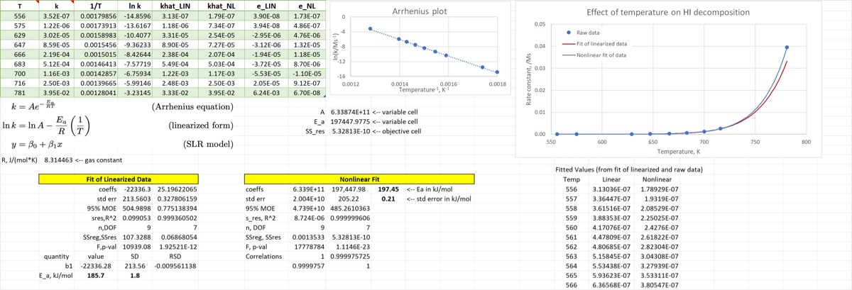
where $R$ is the ideal gas constant. If you perform an experiment in which you measure the rate constant at several different temperatures you have two options if you want to use regression analysis to obtain estimates (with standard errors) of $E_a$ and $A$ : you can perform nonlinear regression to fit the data to the Arrhenius equation, or you can do a linear fit of the data in a so-called Arrhenius plot of $\ln k$ against $1/T$ . Which is better, and why? This screencast examines that question.

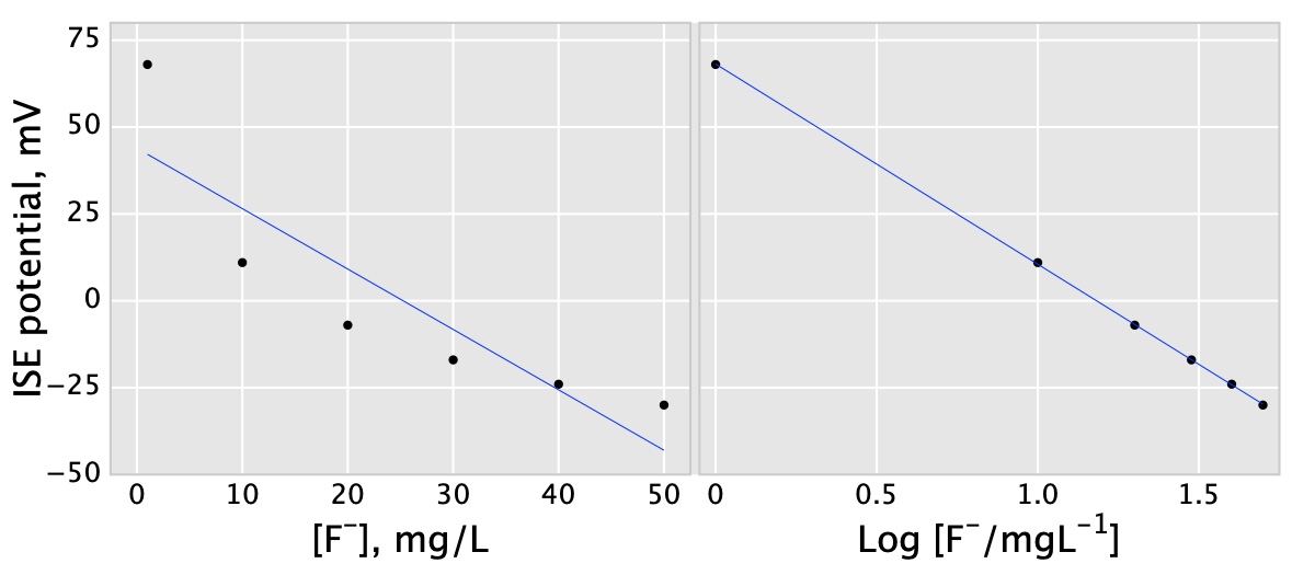
Another example in the screencast is the calibration curve of a fluoride ion-selective electrode (FISE). The FISE is a Nernstian electrode and thus the measured potential is proportional to the logarithm of the analyte concentration. To obtain a calibration curve one will almost always linearize the data by plotting the measured potential against the log of the concentration of a set of calibration standards, as shown below.

Fluoride ISE potential vs concentration is curved and fits a line poorly (left), but vs log concentration it is a straight line (right)

Transformations to Stabilize the Variance

Ordinary least-squares regression assumes homogeneous variance; in other words, it is assumed that the precision of every $Y$ value is the same. There are some cases where that is clearly not the case. One such example, examined in the screencast, is shown below. The image shows repeated measurements of lead calibration standards using anodic stripping voltammetry (ASV).

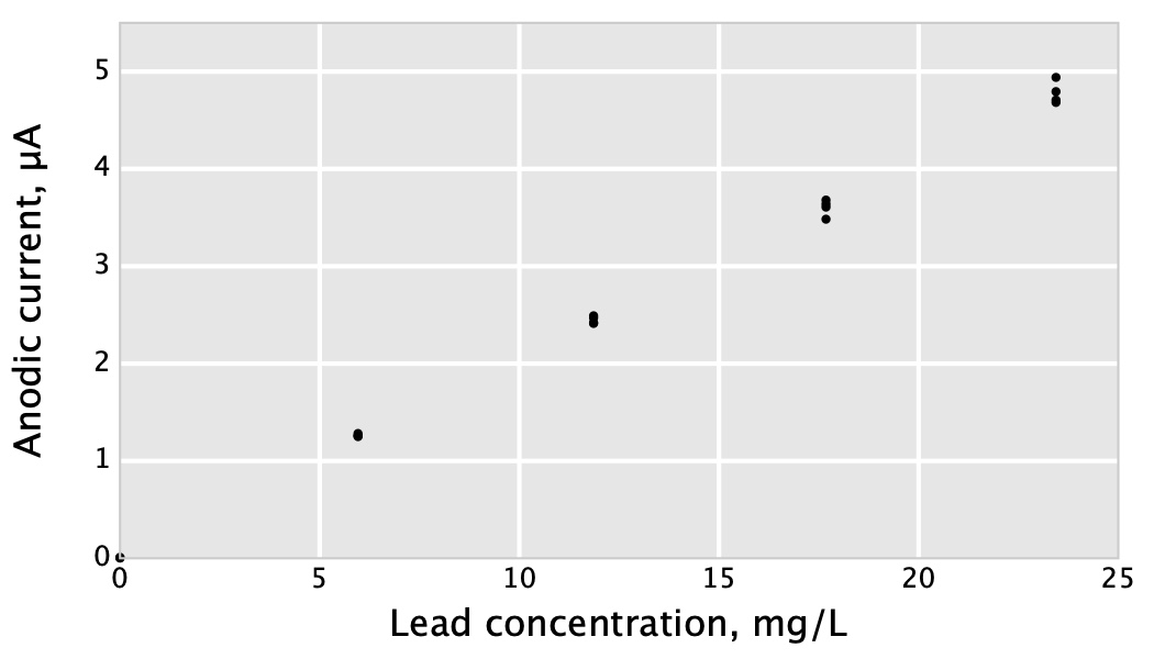
Lead ASV calibration: anodic current vs concentration, with the spread of replicate points growing at higher concentrations

Clearly the spread of the measurements is not the same at different concentrations; in other words the data are nonhomogeneous (or heteroscedastic). Transformations of the variables can result in something more closely approaching homogeneous variance. (Another option is weighted least-squares regression, which will be covered later.)

Learning Goals

Be able to articulate why one would want to transform either $X$ or $Y$ variables (or both)
Be able to explain the effects of variable transformations on regression analysis
Gain more practice doing linear and nonlinear regression as well as error propagation

Tasks

Linearize the Arrhenius data and obtain a best-fit line of the linearized data
From those regression parameter estimates, estimate $E_a$ and its standard error in kJ/mol
Use nonlinear regression to obtain estimates of $E_a$ and its standard error from the raw (ie, not linearized) data
Watch the screencast on the other two worksheets, while taking notes. Then explain which of the two estimates of $E_a$ you would prefer, and defend your choice in terms of the assumptions of regression analysis.

When you are finished, your first worksheet should look something like the image below.

HI decomposition rate vs temperature: a linearized Arrhenius fit (Ea 185.7 kJ/mol) vs a nonlinear fit (197.45 kJ/mol), with both fitted curves plotted

Inverse regression 2 Weighted least-squares regression