Sampling distributions

Download: SamplingDistributions_init.xlsx

Download: Background-Slides.pdf

Introduction

A sample statistic is a value that is calculated from the data in a sample. Since the data have uncertainty, so too do the sample statistics that are calculated from those data. Thus, just like measurements are random variables that must be described in terms of probabilities and probability distributions, the same is true of sample statistics.

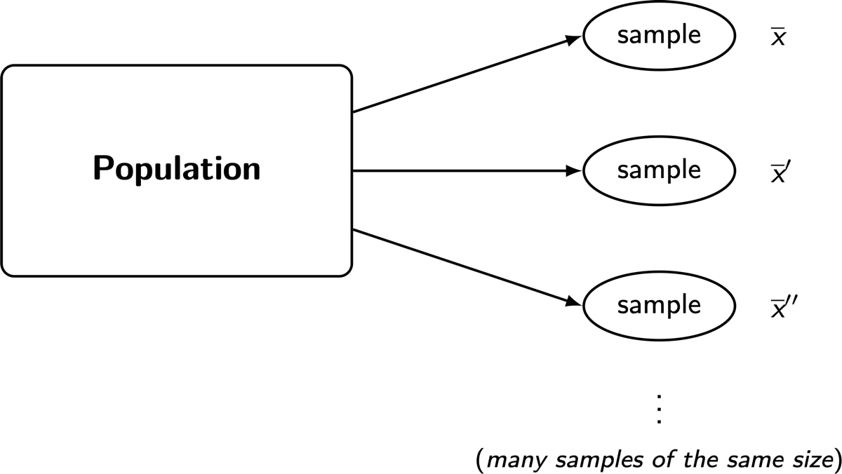
The situation for the sample mean is illustrated below in an image taken from the slides. We imagine a population of all possible measurements of some chemical system. A single experiment consists of taking $N$ measurements that we can average to obtain $\overline{x}$. Imagine repeating that process many times: you will obtain slightly different values of $\overline{x}$ each time. Thus, the sample mean has its own probability distribution (and population for that matter).

The probability distribution of a sample statistic is called a sampling distribution. The standard deviation of that distribution is the statistic’s standard error.

In this screencast we will use simulations to investigate the nature of the distribution of a number of sample statistics.

Learning Goals

• Understand the nature of sampling distributions
• Learn how to use simulations to generate distributions of statistics from some theoretical population
• Learn how the distribution of the sample mean differs from the distribution of the individual measurements
• Learn how properties of the sampling distribution can be used to compare the properties of different statistics
• Understand why the sample variance, calculated by VAR.S in Excel, has a correction factor (the degrees of freedom) in the denominator.

Tasks

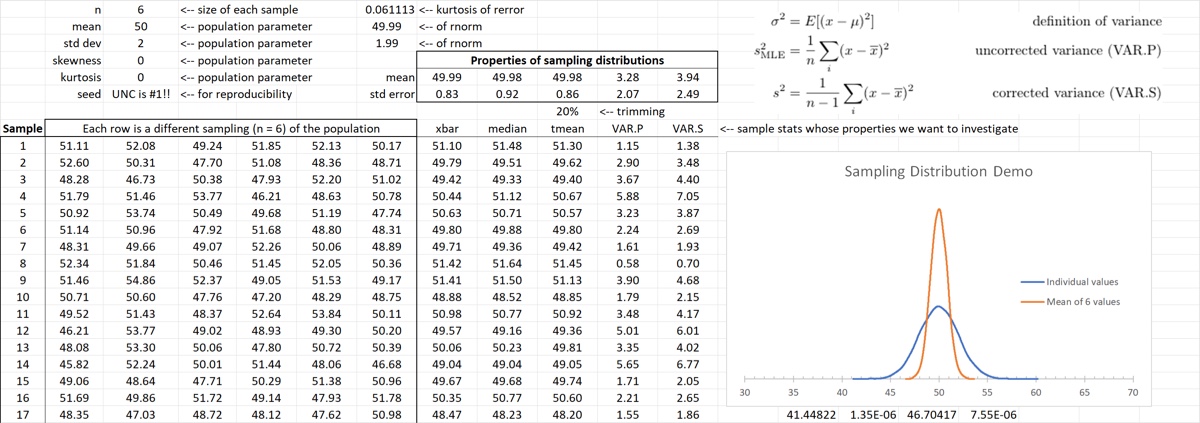
• Name the cells containing the values of the sample count ($n$), and the population values for the mean, standard deviation, skewness, and (excess) kurtosis
• Generate the (seeded) simulation values (1000 draws of six values for each sample) using rerror so that they are sampled from the population with the appropriate mean $\mu_x$ and standard deviation $\sigma_x$
• Calculate the mean for each of the 1000 samples, then compare its distribution to that of the distribution of the individual values using a KDE
• Explore the effect of changing the kurtosis and the skew on the two distributions
• Calculate the median and the 20% trimmed mean for each of the samples. Compare the mean and standard error of the three sample statistics. Explore the effects of increasing kurtosis and skew on those values.
• Calculate the MLE variance (with VAR.P) and the corrected variance (with VAR.S) for each of the 1000 samples, and examine the results to see the trade-offs in using one statistic over the other.

When you are finished your spreadsheet should look something like the figure below.