Regression with SOLVER

Download: RegressionWithSOLVER_init.xlsx

Introduction

In this screencast you will learn to use SOLVER to perform least-squares regression. One reason to do this is to demonstrate the criteria for least squares analysis: it returns parameter estimates (ie, statistics) that minimize the sum of squared residuals. In other words, it minimizes

where $\hat{y}_i$ are the fitted values obtained by using the estimated regression parameters. For the SLR model (best-fit line, which we will be using here),

where $b_i$ is the least-squares estimate of regression parameter $\beta_i$.

Using SOLVER to obtain least-squares estimates is not necessary for linear regression models. A “linear” regression model is one that is linear in the regression parameters; it doesn’t mean that the regression function itself is linear; for example, any polynomial model is a linear model. This distinction will be addressed more thoroughly in a future screencast.

But SOLVER (or a similar optimizing algorithm) is required to perform regression analysis in the following situations:

• any form of nonlinear least-squares regression;
• least-squares regression analysis where one wishes to impose some sort of constraint (eg that the parameter must be non-negative); or
• regression analysis that optimizes some other criterion (ie, not least-squares regression).

So learning to use SOLVER to perform regression analysis will be useful for more than just an illustration of how least-squares regression works.

Learning Goals

• Understand the least-squares criterion in regression analysis
• Learn how to use SOLVER to perform least-squares regression
• Appreciate that the arithmetic mean is a least-squares estimate of location

Tasks

• Calculate the transformed $X$ values to obtain a linear calibration curve: $X = \log C$
• Use SOLVER to obtain least-squares regression parameter estimates. These are steps worth knowing in the future:
  1. Plot the data as an XY scatterplot using symbols
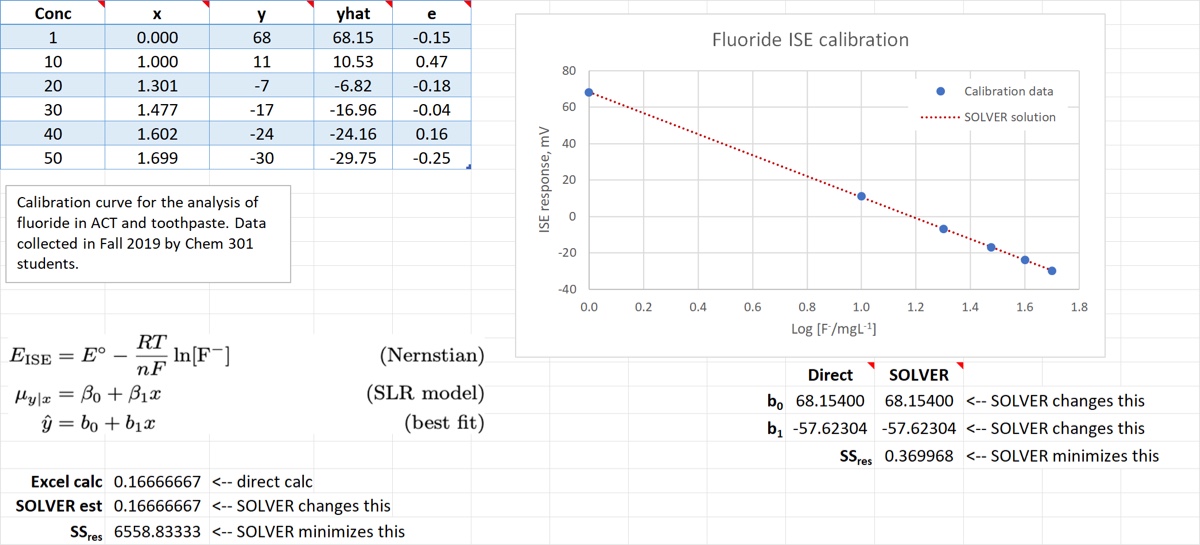
  2. Set up the SOLVER variable cells (ie, the cells SOLVER will change) with initial estimates of the regression parameters. For the SLR model you need to provide initial guesstimates of slope ($b_1$) and intercept ($b_0$).
  3. Using those estimates, calculate the $\hat{y}$ values and add them to the plot as a light line. If necessary, adjust the initial parameter estimates to bring the initial fit closer to the data (but it doesn’t have to be that close).
  4. Calculate the residuals $e_i = y_i - \hat{y}_i$ from the y-hat values you just calculated.
  5. Set the criterion cell formula to be =SUMSQ(e_i) where e_i refers to the range of residuals you just calculated. This is the cell that SOLVER will minimize by changing the variable cells. Confirm that small changes in those variable cells will result in changes to the SSres formula output.
  6. Run SOLVER. You can use the default criteria in most cases but uncheck the box that says “Make Unconstrained Variables Non-Negative”. (Unfortunately that box is checked by default and it shouldn’t be.) After running SOLVER, look at the change in plot and see if the results look good. It doesn’t hurt to return to the SOLVER dialog box and re-run the optimization, just to be sure. If something goes wrong, generate a SOLVER report and examine the log; verify that your SSres cell formula is correct and is responding to changes in the regression parameter estimates. If SOLVER exits abnormally, use the Reset SOLVER routine in the CLS-Stats Utility menu.
• Calculate the slope and intercept values using Excel’s SLOPE and INTERCEPT functions to verify that SOLVER yields the same values.
• Show that the mean is a least-squares estimator: calculate $\overline{y}$ using SOLVER and compare to the value given by the AVERAGE function.

When you are finished, your spreadsheet should look like the image below.