Regression in Excel

Download: RegressionInExcel_init.xlsx

Introduction

Regression analysis is possibly the most common method of statistical analysis. In this screencast we will demonstrate four ways of doing regression in Excel. In all cases we will fit a straight line to some measurement data, sometimes called a simple linear regression (SLR) model:

In regression analysis all uncertainty is assumed to be contained in the $y$ variable and the $\beta_0$ (intercept) and $\beta_1$ (slope) terms are unknown population parameters called regression parameters. The techniques presented in this screencast all return least-squares estimates of these parameters. We will explore the statistical properties of these parameters in future screencasts.

Learning Goals

• Learn some important (native) ways of doing regression in Excel
• Explore three selected CLS-Stats lambda functions related to regression

Tasks

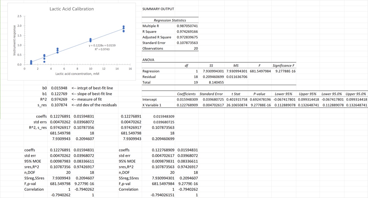
• Plot the data and then add a trendline and display the equation
• Use four simple functions to return SLR least-squares statistics: INTERCEPT, SLOPE, RSQ, and STEYX
• Use the Analysis ToolPak regression procedure
• Use LINEST and label its output.
• Use three CLS-Stats regression functions:
  • LINEST: the CLS-Stats version, a drop-in replacement for Excel’s function that allows for blank values
  • OLS: Performs ordinary least-squares regression, returning more statistics than LINEST and labeling the output
  • PolyLS: A convenient wrapper for OLS for polynomial least-squares regression

When finished your spreadsheet should look something like the image below.