Propagation of error 2

Download: V2-ErrorPropagation2_init.xlsx

Introduction

When we apply the propagation of error partial derivatives method to curved transformations, we are making the assumption that a linear approximation of the function is valid on the scale of the uncertainty. The Monte Carlo (MC) method of error propagation is an alternative method that does not make this assumption, and has a few other added benefits. It is based on simulations and will be illustrated in this screencast.

Learning Goals

Learn how to perform Monte Carlo error propagation in Excel and learn some of its advantages over the partial derivatives method
Understand and be able to explain the consequences of the assumption of linearity in the partial derivatives method

Tasks

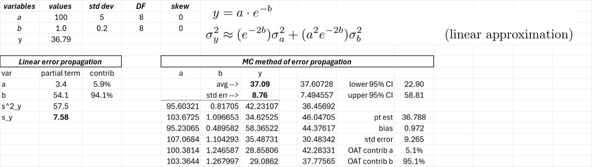
We will assume the following transformation: we have two random variables, $a$ and $b$ , and we are interested in the properties of the random variable $y$ calculated from these two variables as shown below. The estimate of $\sigma_y^2$ using partial derivatives is also shown.

\begin{align*} y &= a \cdot e^{-b}\\ \sigma_y^2\ &\approx (e^{-2b})\sigma_a^2 + (a^2 e^{-2b})\sigma_b^2 \end{align*}

We are assuming here that the two variables $a$ and $b$ are independent. This is a transformation common to many scientific models. In the screencast we will perform the following tasks.

Use rerror to demonstrate how the MC method works
Construct a named callback function to use in the CLS-Stats MC method functions
Use MCM to generate the simulated values and create a QQ plot (against standard normal) of the output
Examine the effect of skew on the output of the simulations
Illustrate the use of MCM_error_V and MCM_CI_V for error propagation

If you follow along with the screencast your spreadsheet should look like the image below.

y = a*exp(-b): linear propagation gives s_y = 7.58, while the Monte Carlo method gives SE 8.76 and a 95% CI of 22.9 to 58.8

Propagation of error 1 Comparison of means