Propagation of error 1

Introduction: Propagation of Uncertainty

If a value $y$ is calculated as a function of a number of random variables, $f(x_i)$ , both the bias and the uncertainty of the result will propagate from the original variables to the calculated result. In this screencast we assume that there is no measurement bias in the random variables $x_i$ ; the uncertainty in the result can be approximated as

\begin{align*} \sigma_y^2\ &\approx \sum_i \left( \frac{\partial y}{\partial x_i} \right)^2 \sigma_i^2\\ &\approx \left( \frac{\partial y}{\partial x_1} \right)^2 \sigma_1^2 + \left( \frac{\partial y}{\partial x_2} \right)^2 \sigma_2^2 + \cdots \end{align*}

This is an approximation because we are assuming that

$y$ is a linear function of the variables $x_i$ (another way of saying this is that we are truncating the Taylor series expansion of the function after the first order). Because of this assumption, this approach is sometimes called linear error propagation to emphasize the fact that when we approximate a curved function with a Taylor series expansion we are retaining only the linear term.
The uncertainties in the variables $x_i$ are not correlated (ie we are not including the covariance terms $\sigma_{ij}$ )

In this screencast you will learn how to apply this method in Excel to determine how the uncertainty (as quantified by the standard deviation) propagates from the source variables to the calculated value. Note that other measures of uncertainty can also be used, such as IQR and MAD.

What is more, the individual terms in the second equation can be used (to a first approximation) to ascribe the variability in calculated value $y$ in terms of the sources of that uncertainty. This will be demonstrated in Excel as well.

The Stepwise (Operations-Based) Method

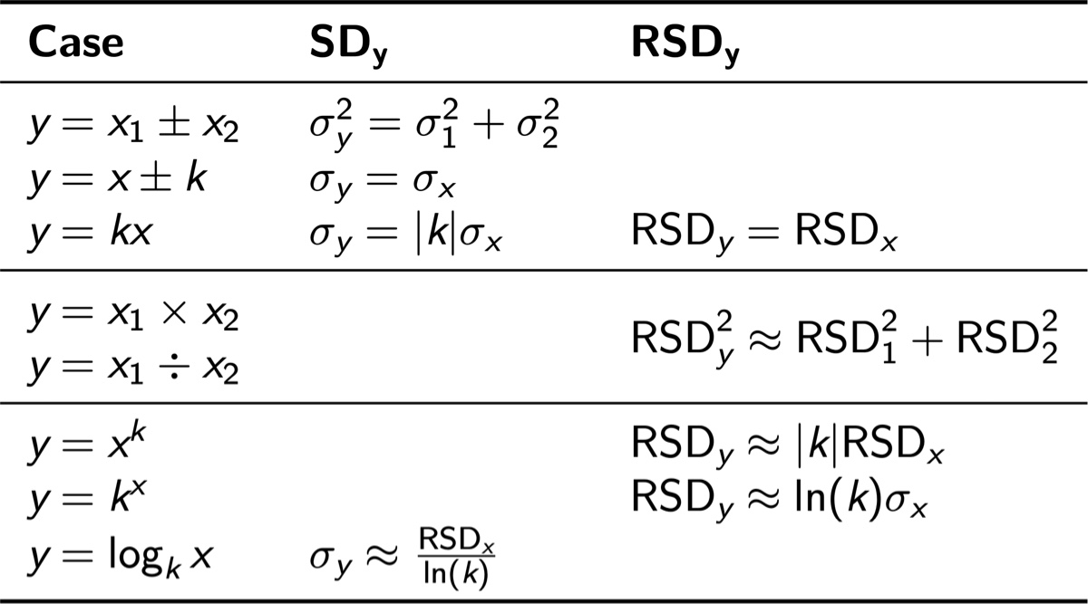
While one can implement error propagation by evaluating each of the partial derivative terms and then summing, another option demonstrated in this screencast is to use an operations-based approach. In this method, the sequence of steps needed to calculate the final result is broken down into a series of operations, and the uncertainty introduced by each transformation is shown in the table below. The entries of this table are determined by the derivative terms, and the same assumptions are made. (It is the same approach, implemented differently.)

Note that some operations-based rules are simpler when expressed as relative standard deviations (or, more generally, relative uncertainty). See the screencast itself for more detail.

Error-propagation rules: variances add for sums, squared RSDs add for products and quotients, RSD scales by |k| for x^k, SD is RSD/ln k for log_k x

Learning Goals

Recognize when (and why) uncertainty propagation is needed
Learn to propagate uncertainty using partial derivatives
Learn to calculate an “uncertainty budget” that estimates how much variability is due to each variable (assuming no interaction effects)
Learn to propagate uncertainty using the stepwise, operations-based method

Tasks

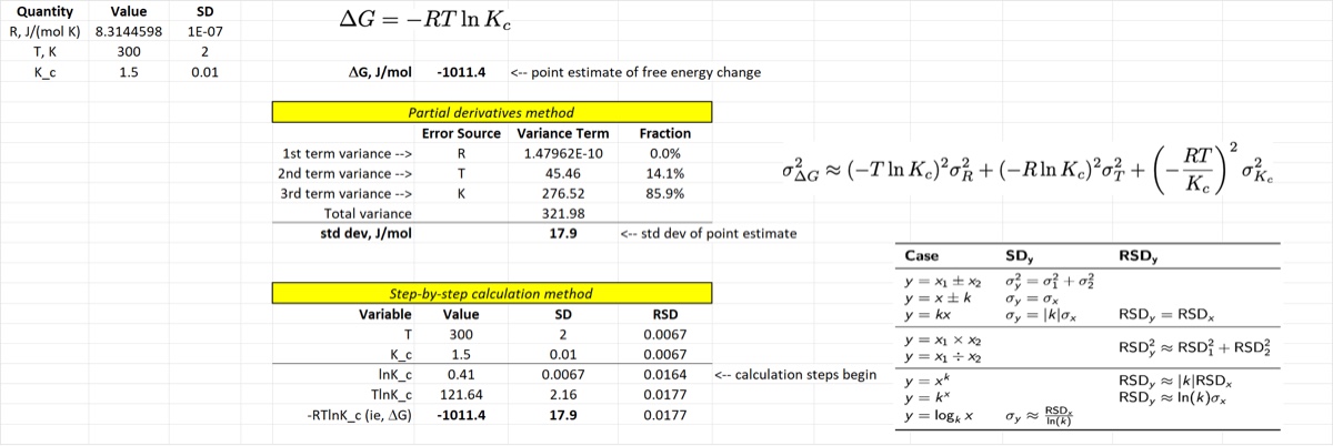
Calculate the value of $\Delta G$ from the three measured values $R$ , $T$ , and $K_c$
Calculate the uncertainty of the $\Delta G$ calculation result using partial derivatives, both directly and using the stepwise method
Partition the variability by input variable. In other words, predict how much of the variability of $\Delta G$ is due to uncertainty in each of the input variables
Note that this partitioning ignores interaction terms that occur in nonlinear transformations. We ignore these interactions when we truncate the Taylor expansion after the first order terms. It is a reasonable approximation as long as the error is fairly small.

Once you are finished with this screencast, your spreadsheet should look something like the image below.

Free energy from Kc: partial-derivative and step-by-step methods both give SD 17.9 J/mol, with Kc contributing 86% of the variance

Propagation of error 2