Propagation of correlated error

Download: PropagationCorrelatedError_init.xlsx

Download: Propagation-of-Correlated-Error-slides.pdf

Introduction

Sometimes when one performs regression analysis, the ultimate goal is to calculate some property that is calculated using two (or more) regression parameter estimates. One such case is the calculation of the optimal flow rate for separation as calculated from the van Deemter equation:

where chromatographic plate height $h$, a measure of separation efficiency (lower is better), is expressed as a function of the flow rate $u$ of the mobile phase. As shown in a previous screencast, one can use linear regression to obtain least-squares estimates of the three parameters $A$, $B$, and $C$. The second equation shows how two of those parameter estimates are used to calculate the optimum flow rate for best separations.

Regression parameter estimates are not independent of one another and so a full propagation of error to estimate the standard error of our calculated $u_\text{opt}$ value must include the correlation between those estimates. In this case, the method of partial derivatives yields

where $\rho_{BC}$ is the correlation coefficient between the two estimates. Note: the approximation symbol $\approx$ is used because this is a nonlinear function that we are approximating with partial derivatives over the range of the uncertainty (first-order Taylor expansion). Although LINEST does not calculate these correlation coefficients, the CLS-Stats regression function OLS returns them so they can be used for error propagation. In this screencast we will illustrate the effect that failure to account for correlation can have in this case; the effects can be significant in some cases (as in this one).

Note that for the situation where $\rho \approx 0$ (or close to it), the cross-terms disappear and we are left with the case of independent error sources.

Learning Goals

• Learn the definitions of covariance $\sigma_{AB}$ and correlation $\rho_{AB}$ (and variable independence)
• Understand why the errors in regression parameter estimates are usually correlated with each other
• Learn how to account for correlation when performing error propagation calculations

Tasks

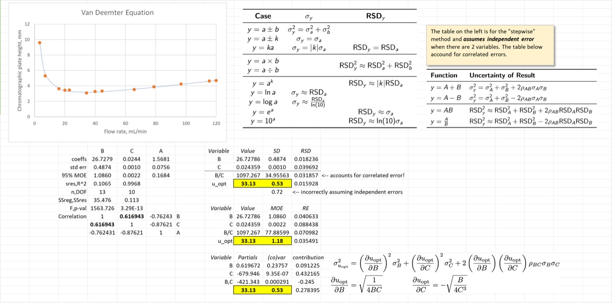
• Estimate the standard error of $u_\text{opt}$ with error propagation using the “stepwise” (calculation-based) method and assuming the errors are independent.
• Estimate the correct standard error of $u_\text{opt}$ by taking correlations into account; use the “stepwise” method
• Estimate the 95% MOE of $u_\text{opt}$ (assumes DOF don’t change)
• Calculate the std error of $u_\text{opt}$ using partial derivatives

At the end of the screencast the first sheet of your spreadsheet should look similar to the image below.