Probability distributions in Excel

Download: ProbabilityDistributions_init.xlsx

Introduction

Measurements are random variables and we have to use the language of probability to draw conclusions about the chemistry system whose properties they are estimating. This screencast demonstrates how to use the theoretical probability distribution functions that are included in Excel.

Probability Distributions in Excel

There are two basic kinds of probability distribution functions (in any language):

• those that accept a quantile as input and return its probability (cumulative or mass/density). In Excel these functions will have .DIST as their extension.
• those that accept a probability as input and return a quantile. In Excel these functions will have .INV as their extension.

Below is a list of distribution functions currently in Excel. Some distribution functions have other convenient extensions (besides .DIST and .INV):

• .2T will return two-tailed probabilities or quantiles (only appropriate for symmetric distributions and currently only available for the t-distribution)
• .RT returns right-tailed probabilities or quantiles

Discrete Distributions

• Binomial: BINOM.DIST, BINOM.INV, BINOM.DIST.RANGE
• Negative binomial: NEGBINOM.DIST
• Hypergeometric: HYPGEOM.DIST
• Poisson: POISSON.DIST

Continuous Distributions

• Normal: NORM.DIST, NORM.INV
• Standard normal: NORM.S.DIST, NORM.S.INV
• Student’s t: T.DIST, T.DIST.2T, T.DIST.RT, T.INV, T.INV.2T.
• Chi-squared: CHISQ.DIST, CHISQ.DIST.RT, CHISQ.INV, CHISQ.INV.RT
• F: F.DIST, F.DIST.RT, F.INV, F.INV.RT
• Log-normal: LOGNORM.DIST, LOGNORM.INV
• Beta: BETA.DIST, BETA.INV
• Gamma: GAMMA.DIST, GAMMA.INV
• Exponential: EXPON.DIST
• Weibull: WEIBULL.DIST

Learning Goals

• Learn how to plot continuous distribution functions (either cumulative or density)
• Learn how to calculate left-tail (LT), right-tail (RT), or interval probabilities for a random continuous variable
• Learn how to calculate quantiles and critical values for a random continuous variable

Tasks

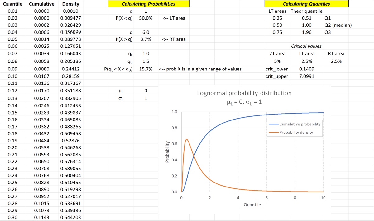
We will use the log-normal distribution because it is asymmetric (meaning no special shortcuts for probability calcs) and because it is commonly used to model some real-world phenomena. All of the tasks are for the standard log-normal distribution $\mu_L = 0$, $\sigma_L = 1$.

• Plot the cumulative probability and probability density of the distribution over a range of 0 - 10 with a step-size of 0.01.
• Verify that the median of the standard log-normal distribution is 1 by calculating the LT area of $x_q = 1$
• Calculate the RT area of $x_q = 6.0$
• Calculate the interval probability $P(1.0 < x < 1.5)$
• Calculate the theoretical first and third quartiles (ie, quantiles $Q_1 = q_{0.25}$ and $Q_3 = q_{0.75}$)
• Calculate the 95% “critical values”, ie $q_{0.025}$ (LT area of 2.5%) and $q_{0.975}$ (RT area of 2.5%)

When you are done with the screencast your spreadsheet should look something like the image below.