Normal distributions

Download: NormalDistributions_init.xlsx

Introduction

In this screencast we explore the properties of random variables that are well described by the Gaussian distribution, a situation common enough that this distribution is called the normal distribution. Measurements tend to be normally distributed when they have many independent sources of variability whose errors are additive. And the probability distributions of many statistics, such as the mean and trimmed mean, tend to be normally distributed (as described by the Central Limit Theorem). So it is important to become familiar with using Excel’s distribution functions to describe the properties of normally distributed variables.

Learning Goals

• learn what the standard normal distribution is and how to calculate its probability density
• learn how to calculate z-scores (quantiles of the standard normal distribution)

Tasks

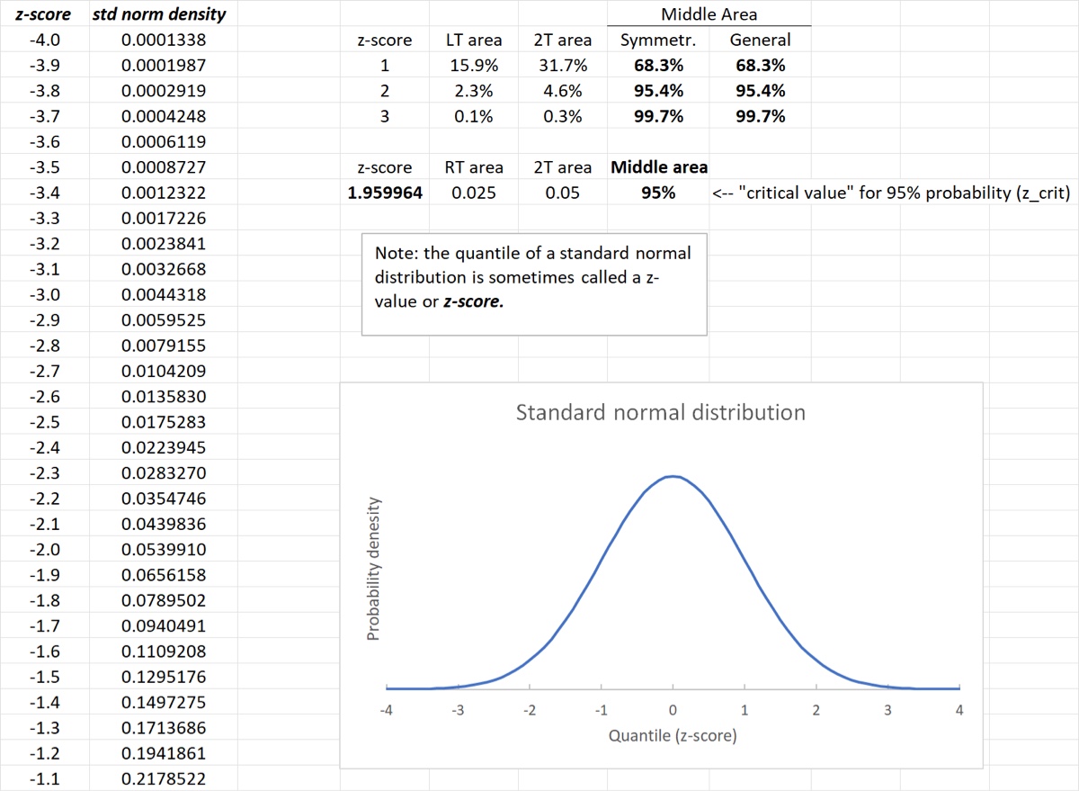
• Calculate and plot the standard normal distribution. Note: the CLS-Stats Series function is a convenient alternative to SEQUENCE for generating the X values of the plot (the screencast uses SEQUENCE)
• Use the standard normal distribution to calculate the probability that any normally-distributed variable is within $\pm 1 \sigma$, $\pm 2\sigma$, and $\pm 3\sigma$ of the mean $\mu$.
• Calculate the z-score corresponding to a 2-tail area of 5%.

When you are finished your spreadsheet should look like the image below.