Nonlinear regression

Introduction

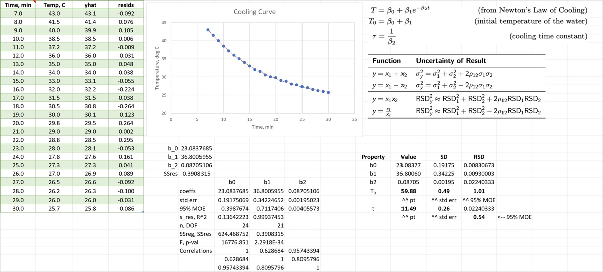
In this screencast we will use a case study to demonstrate how nonlinear regression is performed in Excel with the Nonlinear Regression procedure in CLS-Stats. Specifically, we will fit a cooling curve using Newton’s Law of Cooling:

T = \beta_0 + \beta_1 e^{-\beta_2 t}

where $T$ is the temperature of a cooling body, $t$ is time, and the $\beta_i$ values are regression parameters to be estimated by least-squares regression. This model is nonlinear because the $\beta_2$ term is in the exponent.

The primary goal of the exercise is to estimate the initial temperature $T_ \text{init} = \beta_0 + \beta_1$ of heated water that is cooling to room temperature. While using SOLVER directly would be sufficient to obtain a point estimate, we also want to be able to calculate the standard error and a 95% confidence interval of our result. To do so we need addition regression statistics, which is what the CLS-Stats procedure provides.

You are encouraged to visit the documentation of this procedure before or after doing this screencast. This screencast is also related to a previous screencast that demonstrates how SOLVER can be used to estimate regression parameters but we will review the steps here.

Learning Goals

Learn how to use the CLS-Stats nonlinear regression procedure.
Review propagation of (correlated) error

Tasks

Use the CLS-Stats Nonlinear Regression procedure to obtain LS estimates of cooling curve parameters
Use the results of the regression to calculate a point estimate, standard error, and a 95% CI for the initial temperature of the water
Also estimate the cooling time constant, $\tau$ , as well as its standard error and a 95% CI

When finished your spreadsheet should look something like the image below.

Propagation of correlated error Polynomial regression and model selection