Linear vs nonlinear regression models

Download: LinearNonlinear_init.xlsx

Download: Linear-vs-Nonlinear-Models-slides.pdf

Introduction

When a regression model is linear, it is very easy to find the least-squares estimates of the model parameters as well as the standard errors of those parameters. In contrast, a nonlinear model requires the use of an iterative optimization procedure such as those provided by Excel’s SOLVER. Those are less convenient due to the computational cost of the optimization as well as the need to provide initial estimates. Moreover, in Excel the results are not dynamic; if, for example, you want to add more data or examine the effect of removing an outlier, you have to perform the optimization procedure again. This is not the case with linear LS regression, where the cell formulas can adjust to such changes virtually instantly.

But it is important to understand what exactly is a linear regression model. Importantly, it is not the same thing as a linear function. Consider the van Deemter equation for optimizing chromatographic separation efficiency. It is given by the following equation:

where $h$ is chromatographic plate height (a smaller height means a more efficient separation), $u$ is the linear flow rate, and the $A$, $B$, and $C$ parameters will depend on the nature of the chromatographic instrument. (The parameters have physical interpretations but that is not important for our purposes here.) Below is a plot of the function.

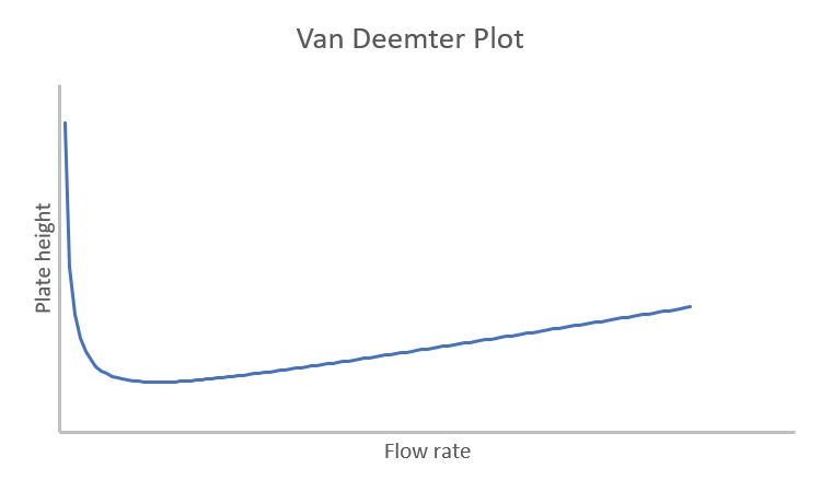
Clearly this is not a linear function, but if we have some data that we want to fit using least-squares regression we would still be using a linear regression model because the function is linear with respect to the regression parameters. A linear regression model is any model that can be expressed in the following form:

where $\beta_i$ is the regression parameter corresponding to independent variable $x_i$. In the van Deemter equation, $A$ is the intercept term ($x_i = 1$), $B$ is the coefficient for the $x_i = \frac{1}{u}$ variable, and $C$ is the coefficient for the $x_i = u$ variable. See the slides (attached above) and the screencast introduction for more examples of linear and nonlinear models.

Learning Goals

• Be able to identify linear and nonlinear regression models
• Use Excel to do regression analysis of a more complicated linear model

Tasks

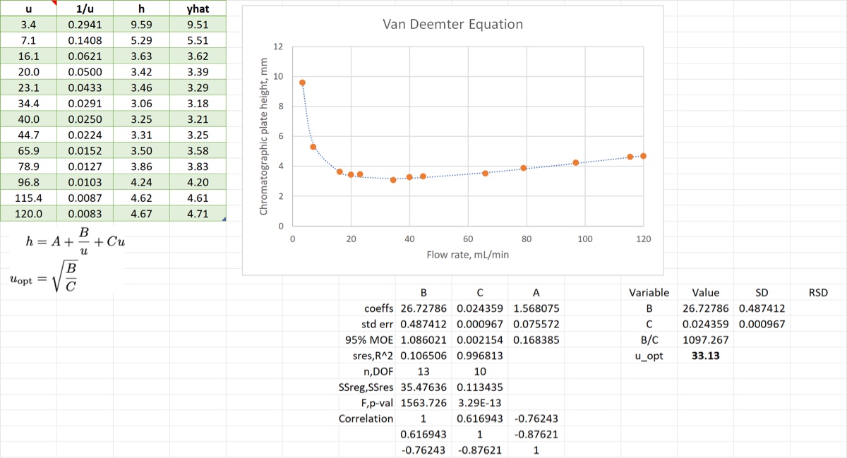
• Convert the data to a table and add a new column to hold the 1/u variable
• Use OLS on the data to obtain estimates of the van Deemter parameters. Identify which column corresponds to which parameter.
• Invoke OLS without using the helper column. (Or just observe and learn about it if you want.)
• Calculate the optimum flow rate and set up an error propagation table that we will use later to find the standard error of this value; see the screencast on propagating correlated error
• Calculate a new table column yhat and add the values to the van Deemter plot to show the fit with the data.

When you finish your spreadsheet should look something like the image below.