Data Visualization

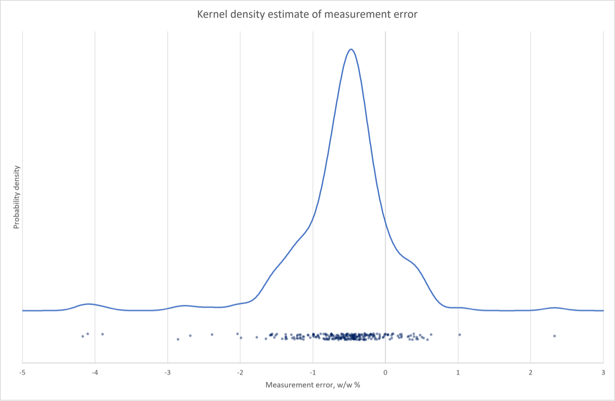
​IMPORTANT NOTE: The interface for the KDE form has been upgraded slightly since this screencast was made, it now allows you to create a horizontal boxplot under the KDE plot, and in fact that is the default. I don’t think it is worth redoing the entire screencast for this feature; I encourage you to play with it and if you would rather do the boxplot instead of the jitterplot that is fine. I would not advise doing both, though; that’s too busy.

• Go to the description of the Kernel Density Estimate (VBA Macro) documentation for more information and an example

Download: DataVisualization_init.xlsx

Introduction

In this screencast you will practice visualizing data distributions using three tools available to you in Excel (with the CLS-Stats add-in loaded):

• histograms
• kernel density estimate (KDE) plots
• boxplots

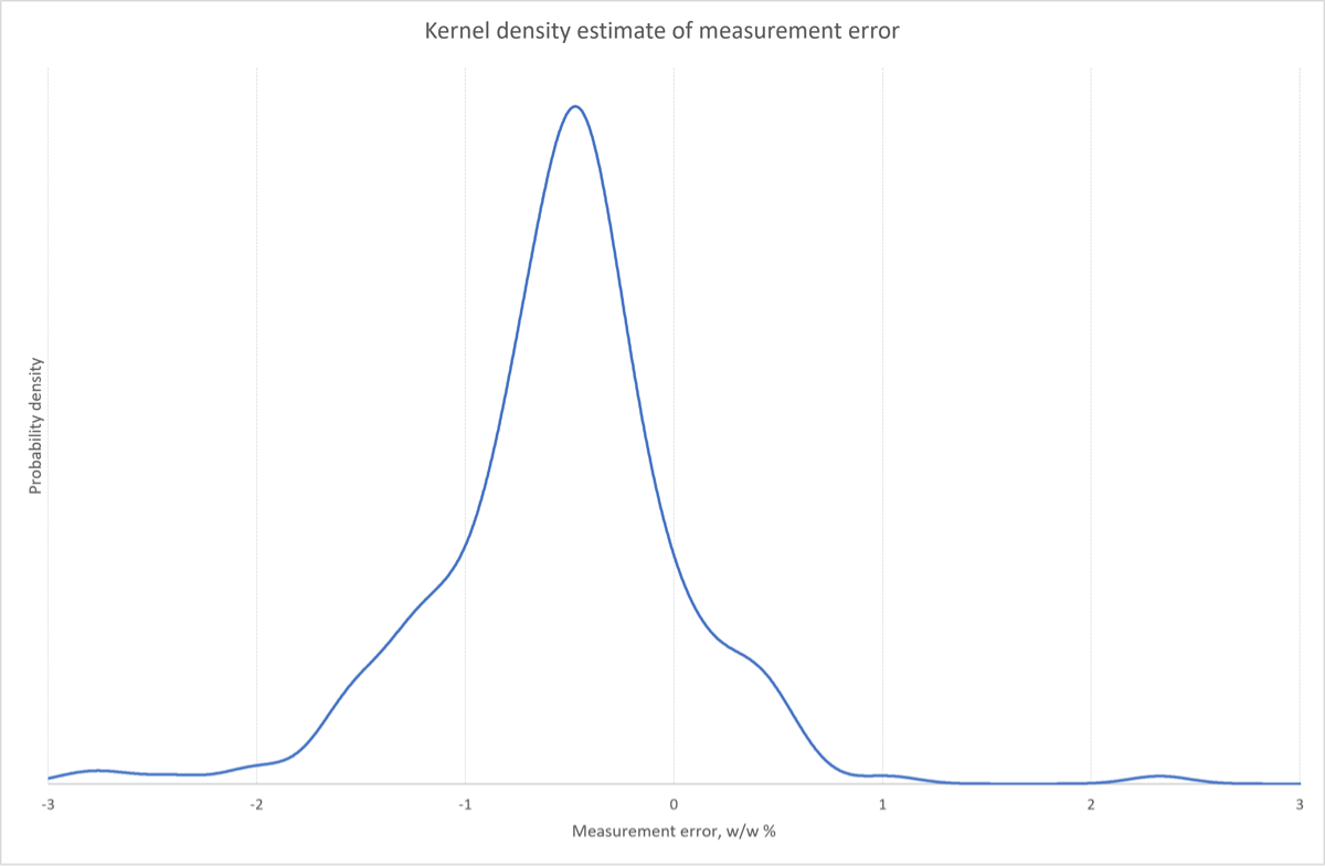
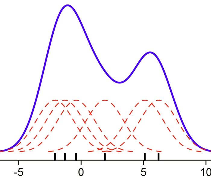
This may be your first exposure to KDE plots. They are essentially alternatives to histograms and are based on the summation of a series of kernel functions centered on each point. They are visualized in the figure below. A larger KDE value means that more points are clustered around that area.

Learning Goals

• Learn how to visualize data distributions with histograms and kernel density estimate (KDE) plots
  • Understand some of the considerations in choosing bin widths (histogram) and bandwidths (KDE)
• Learn how to visualize data with jitterplots and boxplots
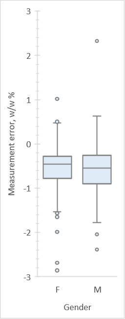
  • Learn the meaning of the components of boxplots
• Learn how to compare distributions of groups with boxplots

Tasks

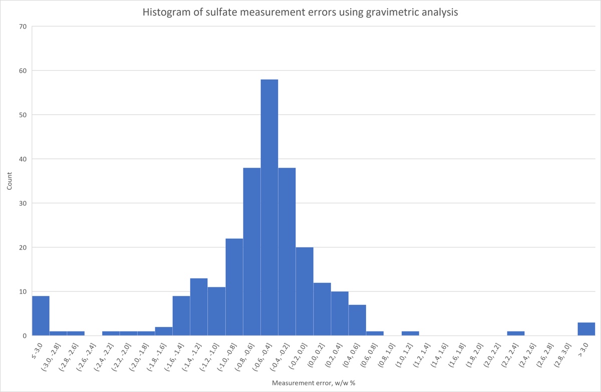
• Create a histogram of the sulfate measurement data using (a) Excel’s histogram plot and (b) L.Hist. Put it on its own sheet. Explore the effects of using different bin widths.
• Calculate the KDE using L.Density and then plot the result on its own sheet. Explore the effect of using different bandwidths.
• Use the KDE macro (Ctrl-Shift-K) to create a KDE with a jitterplot, putting it on its own sheet.
• Recommended (not in screencast): Use the KDE macro to create a KDE with a horizontal boxplot.
• Use boxplots to compare the distribution of measurement errors of males and females.

Below are some of the plots you would produce with this screencast.