ANOVA calcs 2
Download: ANOVA_Calcs2_init.xlsx
Introduction
ANOVA partitions the total variability into two types: between-group and within-group variability: where
The sum of squared deviations of the group means from the overall (grand) mean is scaled by multiplying by the number of measurements in each group. This is so that the between-group variability is “applied” to each observation rather than each group.
The between-group mean square, (where is the number of groups), estimates the following population parameter
In this equation, is the effective group size, a weighted average that is usually very close to the (unweighted) average group size.
If all groups have the same number of measurements then we can simplify the expression to and . This is called a balanced design ANOVA and is preferred for a few reasons:
- it makes it easier to detect (in a statistical sense) the presence of between-group variability. In other words, it maximizes the statistical power of ANOVA
- it makes ANOVA more robust to deviations from the assumptions of normality and homogeneous variance
But unbalanced designs happen all the time; for example, individual trials/observations/measurements can go awry or data are simply missing. In such cases the effective group size, which is slightly less than the average group size, is the scaling factor that accounts for the contribution of the between-group variance to .
Learning Goals
- Understand the advantages of balanced designs in ANOVA
- Learn how to create dynamic named ranges in Excel
Tasks
- Make the following named ranges dynamic:
Group,xbar_i,s_i - Make the following named ranges dynamic:
ANOVA_data,n_i - Calculate
w_icolumn and name it - Calculate effective group size and interpret its meaning
- Examine the effects of balanced vs unbalanced designs for different values of
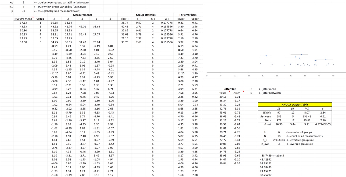
By the end of the screencast your spreadsheet should look something like the image below.