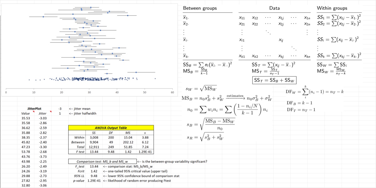
ANOVA calcs 1

Introduction

Variability Partitioning

In ANOVA observations belong to a group. In one-way ANOVA the grouping only goes one level deep; you can also have sub-groups and sub-sub-groups. The structure of the data is shown in the image below. You can imagine the data as a table in which the rows correspond to different groups and the columns correspond to different observations or measurements. So measurement $x_{ij}$ refers to the $j^{\text{th}}$ measurement in the $i^{\text{th}}$ group.

Layout of one-way ANOVA data: group means, the data table, and within-group sums of squares, with formulas for SS_B, SS_T, SS_W and SS_T = SS_B + SS_W

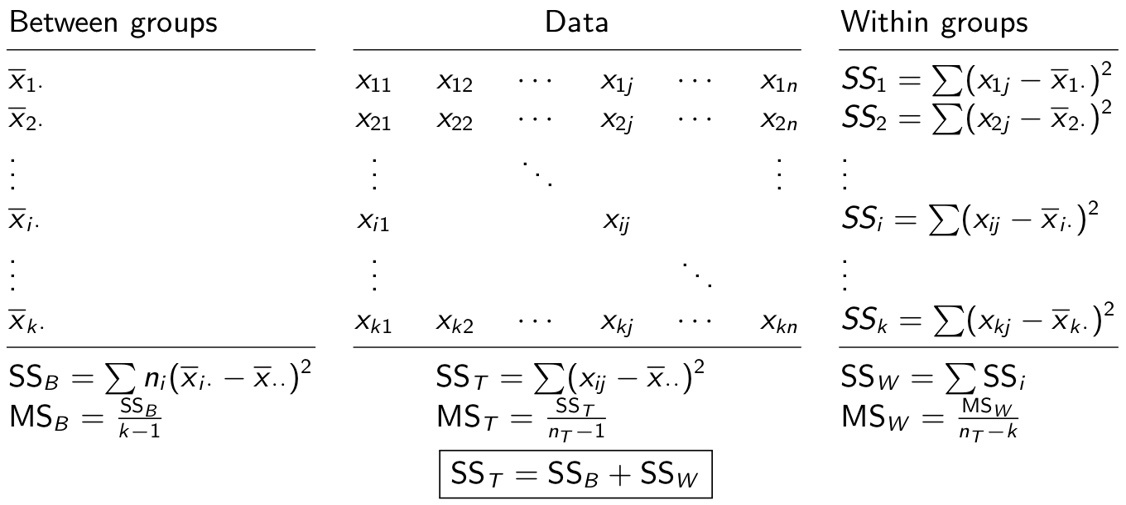
ANOVA famously has a lot of equations (though they are represented more simply using matrix algebra). The sum-of-squares (SS) terms are all sums of squared deviations from a mean of some kind. They measure unscaled variability. Greater deviation from the mean leads to larger SS values but it is “unscaled” because they are additive and adding more groups and measurements will increase them even if the underlying sources of variability do not change. The $\text{SS}_T = \text{SS}_B + \text{SS}_W$ is the key equation that partitions the variability into two sources: that due to changing group properties (between-group variability, $\sigma_B$ ) and that due to measurement or observational uncertainty (within-group variability, $\sigma_W$ ).

The equations below show how ANOVA can provide estimates of those two sources of variability. The estimate of $\sigma_W$ is the pooled standard deviation; it assumes homogeneous variance meaning that it assumes all measurements share the same measurement variability. The estimate of $\sigma_B$ is based on the difference between the $\text{MS}_B$ and $\text{MS}_W$ terms.

\begin{align*} s_W &= \sqrt{\text{MS}_W} \\ \text{MS}_B &= n_0 s_B^2 + s_W^2 \xrightarrow{\text{estimates}} n_0 \sigma_B^2 + \sigma_W^2 \\ n_0 &= \sum w_i n_i = \sum \left( \frac{1 - n_i/N}{k-1} \right) n_i \\ s_B &= \sqrt{\frac{\text{MS}_B - \text{MS}_W}{n_0}} \\ s_R &= \sqrt{s_B^2 + s_W^2} \end{align*}

Significance Testing

Significance testing is based on a one-sided confidence “interval”: a lower confidence bound of a comparison statistic. That statistic is the ratio of the between-group and within-group mean square values.

\frac{\text{MS}_B}{\text{MS}_W} \xrightarrow{\text{estimates}} \frac{n_0 \sigma_B^2 + \sigma_W^2}{\sigma_W^2}

If there is no between-group variability (ie, if $\sigma_B = 0$ ) then this statistic is estimating the ratio of two independent estimates of the same quantity, $\sigma_W$ , and should be statistically indistinguishable from 1. The usual practice is to calculate a lower confidence bound; if that boundary is larger than 1 then there is confidence that the comparison statistic is significantly greater than 1. (The reason this is a one-tailed test is because $\sigma_B^2 \ge 0$ since variances cannot be negative.)

Learning Goals

Develop an intuitive grasp of the ANOVA equations that partition variability between its sources
Learn how to do ANOVA calculations in Excel
Be able to interpret the output of ANOVA calculations

Tasks

Review the ANOVA data structure
Review the ANOVA equations, defining terms
Perform ANOVA calculations using ANOVA1S and ANOVA
Interpret each item in the ANOVA table output

When finished your spreadsheet should look something like the image below.

Group means with error bars and a jitterplot, ANOVA formulas for s_W, s_B and n_0, and an ANOVA table with F = 13.44, p = 1.3E-41

ANOVA demonstration ANOVA calcs 2