Nonlinear Regression

Keyboard shortcut: Ctrl-Shift-N

Description

This VBA procedure uses Excel’s SOLVER to obtain least-squares parameter estimates for nonlinear regression models. While it can be used for any regression model, it is intended to be used for nonlinear models (ie, models that are nonlinear functions of regression parameters) since linear regression can be performed with Excel’s LINEST and the CLS-Stats regression functions OLS and PolyLS.

Note that even though this procedure is named “Nonlinear LS Regression” in fact it can be used for any regression model.

Use

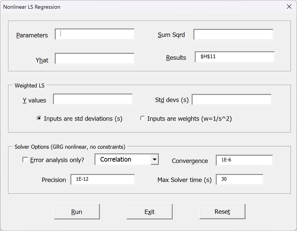
Below is the form that appears when you select this nonlinear least-squares (NLS) regression procedure from the ribbon menu (or press Ctrl-Shift-N).

• The Parameters are the regression parameters that SOLVER will alter in order to obtain the least-squares estimates. There need to be initial estimates in those cells; it is recommended that you plot both the data and the fit (calculated using these parameters) so that you can know that you are reasonably close to the true value.
• The Sum Sqrd field points to a single cell that contains the sum of squared residuals, $SS_{res}$, that are calculated with the parameters you just selected. You should check to make sure that changing the parameters slightly will also change the $SS_{res}$ value, because that is how SOLVER will find the LS estimates: it will explore the surface of $SS_{res}$ as a function of the Parameters cells until it finds a minimum.
• Yhat contains the address of the fitted values $\hat{y}$ calculated from the regression model. These values are used to calculate the uncertainty statistics and correlation/covariance matrix. You’ll probably also be using them to calculate the residuals and will probably be plotting these values to assess the fit visually.
• Results points to the upper left cell of the output from the procedure. If the output will overwrite some data you will be warned about it and have the option to change the location of the output.

The second group of inputs are used if you wish to perform a weighted least-squares fit.

• In this case it is up to you to include the weights appropriately in the Sum Sqrd cell formula. Typically you will use a cell formula that returns a value corresponding to $\sum w_i e_i^2 = \sum e_i^2 / s_i^2$, where $w_i$ are the weights of each residual $e_i$ for the fit and $s_i$ is the estimated standard deviation of the $i^\text{th}$ data point.
• You can input either the weights or the standard deviations. Inputting the $Y$ values allows for some error checking to see if the fit is consistent with the provided weights or standard deviations.

For most cases you will leave the third set of controls at their default values. Here is what they mean:

• If the checkbox is checked then SOLVER is not actually invoked at all; the current values of the parameters are accepted as correct. Instead the routine performs an “error analysis” on those values to determine their standard errors and parametric margins of errors (MOEs), as well as calculating some other regression statistics like the standard deviation of the residuals ($s_\text{res}$) and coefficient of determination ($R^2$). This is appropriate if you have already invoked SOLVER to find the solutions (possibly to generate a SOLVER report) and simply want the rest of the regression statistics that this procedure supplies.
• Similar to OLS and PolyLS this routine will return either a correlation matrix or a covariance matrix. Use the dropdown to choose which you want to use.

The last three options are fed directly in the call to SOLVER; please check out Frontline’s documentation for more information; the SOLVER stopping conditions page is particularly pertinent. SOLVER returns when one of the following conditions is met:

• The relative change in $\text{SS}_\text{res}$ does not change by more than the Convergence value on successive iterations; so the default value of 1E-6 means that the value changes by less than one part per million over successive iterations.
• The absolute value of $\text{SS}_\text{res}$ does not change by more than the Precision value on successive iterations; this is a closeness tolerance.
• The maximum time is reached.

Click the Run button once you are ready. The dialog will not disappear after SOLVER finds a solution (assuming it does). You are encouraged to run the procedure again, watching the fit and the $SS_\text{res}$ value to make sure it does not change (sometimes SOLVER needs a couple iterations to zero in on the solution if the function surface is fairly flat). Click Exit (or hit the ESC key) to dismiss the window once you are finished.

​The results of the calculation are static and are similar to the results from the regression lambda functions OLS or PolyLS: it is a labeled table with the LS estimates of the coefficients, the standard errors of those estimates, the parametric 95% CIs, and other statistics. See the documentation for OLS for more details (or the example below).

Because the results are static, if anything changes (new data, altered data) you will have to run the Nonlinear Regression routine again to get updated estimates.

Examples of unweighted and weighted nonlinear LS regression

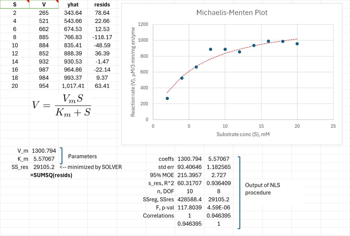
The first example is used to illustrate how to use nonlinear regression to fit data to the Michaelis-Menten equation, where reaction rate $V$ is modeled as a function of substrate concentration $S$. Here is a suggested procedure for obtaining the LS estimates for the parameters of this nonlinear regression model.

1. Plot the data in an XY scatterplot.
2. Create cells for each parameter (in this case the $V_m$ and $K_m$ terms) and enter initial estimates of the values. This can be the most daunting part of the procedure. A physical interpretation of the parameters can be helpful, as well as a fit of the linearized model. In the case of Michaelis-Menten kinetics, we know that $V_m$ is the maximum reaction rate, which looked to be about 1000 units, and $K_m$ is the concentration it takes to get to half-maximum, which looked to be about 5 mM.
3. Calculate the fitted value, $\hat{y}$, from those initial estimates using the regression model. That is the yhat column in the figure below.
4. Add the fitted values to the plot as a line. If needed, alter the parameters to improve the fit but don’t be too obsessive about it. As long as you are reasonably close SOLVER will find the solution.
5. Calculate the residuals, $e_i = y_i - \hat{y}_i$, as the difference between the observed and fitted values. Those are in the resids column below; the cell range is named.
6. Create a cell and calculate the sum of squared residuals, $SS_\text{res} = \sum e_i^2$, which is what SOLVER will minimize. Excel’s SUMSQ function is good for this. At this point your Excel worksheet should look something like the figure above.
7. Verify that small changes to each parameter will produce a change in $SS_\text{res}$ and in the visual fit. Then call the Nonlinear Regression routine, point the inputs to the appropriate cells, and click Run and assess the results: the visual fit should look noticeably better and $SS_\text{res}$ should have decreased. Run it again before closing the window to make sure SOLVER found the solution.

The image below shows the results of clicking Run with the setup in the previous figure. It is in the first worksheet of the Excel file attached below.

The next example (the second worksheet in the file below) illustrates the use of weighted nonlinear regression to determine the temperature of a blackbody radiator. The data were collected by the FIRAS Michelson interferometer aboard NASA’s Cosmic Background Explorer satellite. The results are shown in the image below. The plot on the left shows the fit of the data to Planck’s Law while the plot on the right shows how the measurement standard deviations are much higher for the low-brightness measurements. Using weighted least-squares provides better estimates of the standard errors of the parameter estimates, and ultimately better estimates of the blackbody temperature. These standard errors are not just lower – this is typical, provided that the estimates of standard deviations are not too noisy – but the estimates themselves are more accurate.

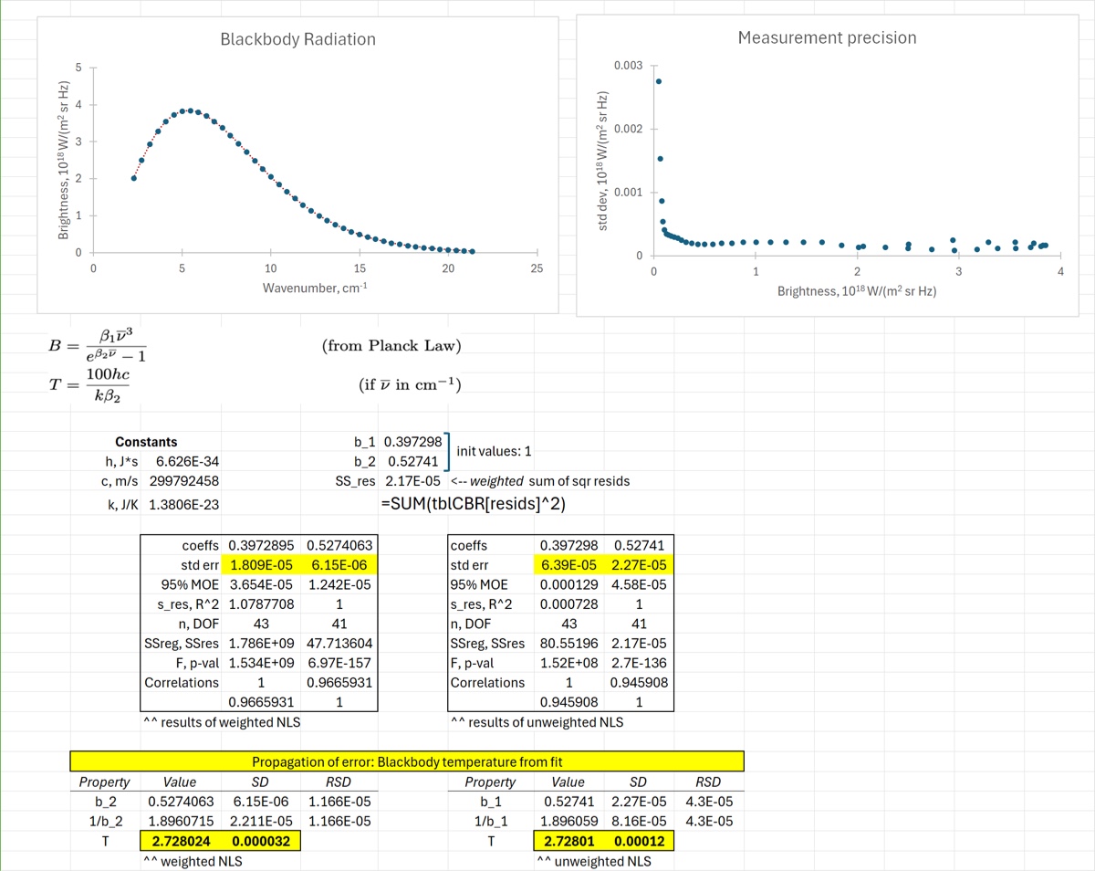
Note: as an estimate of the cosmic microwave background temperature, the result here is far too precise because it does not adequately reflect all sources of variability and systematic error. A recent estimate put the value at $2.7260 \pm 0.0013$ K, where the uncertainty is largely due to uncertainty in systematic measurement error.

Download: NonlinearRegression.xlsx