Inverse Regression

Keyboard shortcut: Ctrl-Shift-I

Description

The Inverse Regression VBA procedure performs inverse polynomial regression using Excel’s SOLVER and returns exact 95% confidence intervals for any polynomial order. It has the same goal as the PolyInv lambda function, which now does everything this procedure does (orders 1-5, exact limits for weighted and unweighted fits) without SOLVER and recalculates when the data change; this procedure’s output is static and it must be run again if the input data or the order change.

Background

Given a measurement on an “unknown” concentration ($y_u$), the predicted concentration $\hat{x}_u$ is obtained by finding the appropriate polynomial root of the polynomial fit to the calibration data. The upper and lower 95% bounds are the points at which the upper and lower 95% prediction intervals (PI) of the calibration fit are equal to $y_u$. These three points are illustrated in the figure (using the data in the Example below).

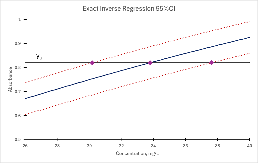
One caveat: one or more of these points might be undefined because $y_u$ never intersects the curve. It is possible that all three are undefined.

In the Inverse Regression VBA procedure, SOLVER is used to find all three of these points from reasonable starting estimates. The procedure also provides a mechanism by which you can assess whether SOLVER fails to find a solution (almost certainly because one doesn’t exist).

Use

If you select the Inverse Regression item from the ribbon, or use the Ctrl-Shift-I keyboard shortcut, the following form appears.

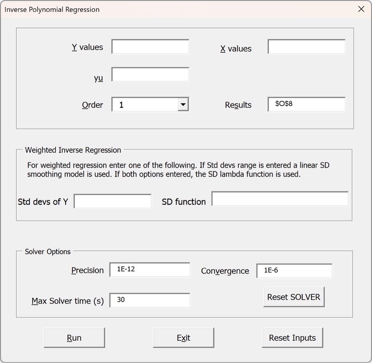
• the X and Y inputs are the addresses of the cells that hold the independent and dependent variables, respectively. Since this is usually a calibration curve, X will be concentration and Y will be the measured signal
• the yu input either points to the cell holding the measured value of the solution whose concentration we want to estimate, or you can enter that value directly into the form (instead of the cell address).
• the Order is an integer value for the polynomial order. The allowed values are 1 - 5.
• the Results field points to the upper leftmost cell of where the results will be. The results are a $6 \times 4$ labeled table; if that will overwrite anything you will get a warning.

The Weighted Inverse Regression group has two inputs; you only need to enter ONE of them. (If both are used then only the second input is used.)

• The first input is a range of cells (or a named range) containing the standard deviations of the $Y$ measurements. A linear model (with intercept) will be fit to these standard deviations as a function of the measurement ($Y$) values and used with PolyPred to find the confidence interval.
• The second input is a named or inline lambda function. The main purpose of this input is if you want to use a model of measurement precision OTHER than “linear fit with intercept.” You can write the function in the input box; for example, LAMBDA(y,b_1*Y) would use a linear model without an intercept using named slope value b_1.

The Solver Options group has three inputs that control SOLVER stopping conditions.

The output is a labeled table like that shown in the example below. The first and last columns are labels. The second column contains the results:

1. Order (for labeling purposes, because you have no cell formula to remind you)
2. The point estimate $\hat{x}_u$ obtained by SOLVER determining the root of the polynomial with $y = y_u$
3. The standard error of the point estimate. This is an approximate value calculated by error propagation: dividing $s(e_u)$ – the standard error of the residuals at $x = \hat{x}_u$ – by the slope of the polynomial at $x = \hat{x}_u$
4. The 95% parametric margin of error, obtained by multiplying $t_\text{crit}$ by the standard error.
5. The lower and upper boundaries of the 95% confidence interval. These are exact values, obtained by SOLVER determining where $y_u$ crosses the lower and upper boundaries of the 95% prediction interval.

The third column contains the following information:

1. The value of $y_u$ input into the procedure (as a reminder).
2. The value predicted by substituting $\hat{x}_u$ into the polynomial. It should match the value above it if SOLVER found the root. The comment in the label to its right (in the fourth column) is also the message from SOLVER after it finished. Hopefully it says that it found a solution.
3. The third value is the slope of the polynomial as calculated by the PolySlope lambda function. It is used to calculate the (approximate) standard error and MOE values using error propagation.
4. The fourth value is the DOF of the standard error (should be $n - p - 1$ where $n$ is the number of data points and $p$ is the polynomial order).
5. The last two values are SOLVER solution checks for both (exact) CI boundaries. The pattern is the same as for the check on $\hat{x}_u$: the value should match $y_u$ and the comment in the neighboring label should report that SOLVER found a solution.

Regarding the solution checks: if everything is going well then $y_u$ should cross three lines: the two 95% prediction interval boundaries and the fitted calibration curve. If $y_u$ crosses those three curves then SOLVER should find a solution. But it can definitely happen that only SOME of those curves are crossed. For example, if the 95% PI is very wide then its lower boundary (for a monotonically increasing calibration function) might not cross $y_u$. In that case SOLVER fails to find a solution because it doesn’t exist and there is just one confidence bound. And of course it could easily be that the calibration curve reaches a maximum that is lower than $y_u$ and so no point estimate is found. Visual examination of the calibration curve and mental comparison of $y_u$ to those values is a useful sanity check.

Example

We can illustrate with the example below: an instrument (flame AA) is used to create a calibration curve for copper and then performs inverse regression. The outputs of the inverse regression routine are at the bottom for two orders. The yellow highlighted cells compare the CI boundaries predicted by the VBA routine (found with SOLVER) with the values predicted by PolyInv, which only finds approximate values for a quadratic fit.

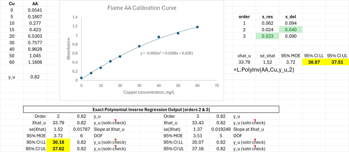
Perhaps more importantly: if one or more of the CI boundaries is not defined, the VBA routine will flag that because the diagnostics in the output will show that SOLVER failed to converge on a solution. But PolyInv will happily predict a solution for a quadratic fit even if it is not defined.

Note that PolyInv does in fact produce an exact CI for the case where a best-fit line is the appropriate calibration function. It might be useful to run the VBA routine just to confirm that you are using it correctly, but there is no reason to prefer it to the dynamic PolyInv output.

Download: InverseRegression-VBA.xlsx