PolyInv

Description

PolyInv performs inverse regression for a polynomial fit of order 1 to 5: it estimates the x value $x_u$ corresponding to a new measurement $y_u$ that was not part of the original calibration. It can do this for either ordinary or weighted least-squares regression; for best accuracy with weighted LS models it is recommended that an SD fitting model is supplied to the function.

Background

Inverse regression is when one attempts to predict an $x_u$ value from a measured $y_u$ value using a calibration curve (a series of measurements of known concentrations). This is sometimes called the “calibration problem.” The resulting prediction, $\hat{x}_u$ , has uncertainty because of the uncertainty in $y_u$ as well as the uncertainty in the regression parameter estimates obtained by fitting the calibration curve data.

The standard error is obtained by error propagation, dividing $s(y_u)$ by the slope of the calibration curve at $x = \hat{x}_u$ . The confidence interval limits are obtained where the prediction band limits are equal to $y_u$ . We can obtain exact solutions for unweighted best-fit lines using Fieller’s theorem, giving the following equations.

\begin{align*} \hat{x}_u &= \frac{y_u - b_0}{b_1} \\ g &= \left(\frac{t_\text{crit}\cdot s({b_1})}{b_1}\right)^{2} \\ x_{U,L}\ &= \hat{x}_u + \frac{g(\hat{x}_u - \bar{x}) \pm \dfrac{t_\text{crit} \cdot s_{\mathrm{res}}}{|b_1|}\sqrt{\left(1+\dfrac{1}{n}\right)(1-g) + \dfrac{(\hat{x}_u - \bar{x})^{2}}{S_{xx}}}}{1-g} \end{align*}

Note that the CI boundaries are not quite centered on point estimate $\hat{x}_u$ but they should be pretty close to $\hat{x}_u \pm s(\hat{x}_u)$ in most cases.

For higher order polynomials, and for weighted polynomial regression of any order, when sd_fn is provided the function uses numerical root finding to determine the points where the 95% prediction bands cross the value of $y_u$ ; the $x$ values corresponding to those points are the lower and upper bounds of the 95% confidence interval for the true value of $x_u$ that produced the measured value $y_u$ . Approximate values for the standard error and 95% margin of error (MOE) are also returned by the function; these are estimated using a first-order Taylor expansion (delta method).

Syntax

PolyInv(Y, X, yu, [p=1], [sd_fn], [S], [s_u]) where

Y and X are the dependent and independent variables, as either row or column vectors
yu is the measurement at which to perform inverse regression
p is the polynomial order, which defaults to p = 1; integers of up to p = 5 are allowed.
sd_fn is the optional model of the standard deviations as a function of Y, as a lambda; eg LAMBDA(y, 0.05+0.3*y) for a linear fit of SD
S is the vector of standard deviations of Y (ignored if sd_fn is supplied)
s_u is a scalar describing the standard deviation of yu (ignored if sd_fn is supplied, required if S is supplied)

The function returns five values:

The best-fit value $\hat{x}_u$ obtained by inverting the regression model (ie, solving for X given Y).
The approximate standard error of $\hat{x}_u$ , ie $s(\hat{x}_u)$
The approximate 95% MOE of $\hat{x}_u$ , which is calculated as $t_\text{crit} \cdot s(\hat{x}_u)$
The lower limit of the 95% CI (exact)
The upper limit of the 95% CI (exact)

The last two values do not coincide exactly with $\hat{x}_u \pm t \cdot s(\hat{x}_u)$ , though they are usually pretty close.

Note that there are some cases where $y_u$ never crosses the upper or lower prediction boundary, or even the best-fit polynomial. In such cases a value of undefined is returned in place of a numeric value.

Example

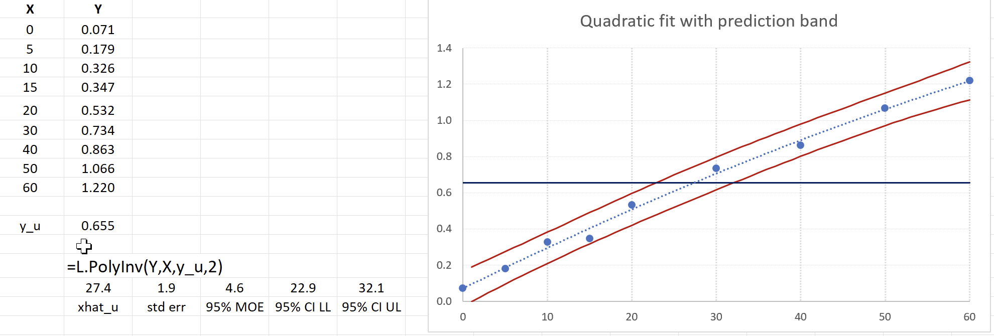
The example below shows how PolyInv is invoked (the X, Y, and y_u ranges are named) for a quadratic calibration curve. The result of the inverse regression might be reported as $27.4 \pm 4.6$ . The confidence interval boundaries coincide with where the blue horizontal line (at $y_u = 0.655$ ) intersects the prediction band lines.

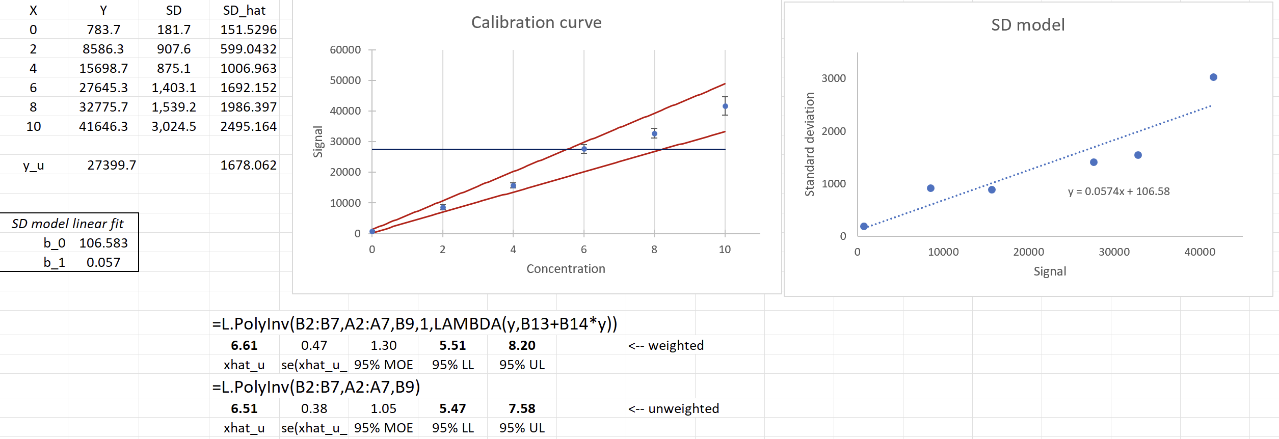
Quadratic calibration with prediction band; the line y_u = 0.655 crosses it to give PolyInv x_u = 27.4, CI 22.9 to 32.1

The next example, which is in the second worksheet of the Excel file below, shows how weighted least-squares might be used with inverse regression. Note that, for best results, two models are needed: the usual model of the response variable (Y) as a function of the independent variable (X), and a model of the response precision ( $s_y$ ) as a function of the response magnitude. The results of weighted and unweighted inverse regression are compared; the main difference is the upper bound of the confidence interval, and it is clear from the figure that the intersection of $y_u$ and the lower prediction boundary is better described by the weighted version of the PolyInv call.

Calibration with SDs that grow with signal and a linear SD model; weighted PolyInv gives 6.61 (5.51 to 8.20), unweighted 6.51 (5.47 to 7.58)

Download: PolyInv.xlsx

Source Code

Helpers used: _Bisect, _InvLimit, _PolyFit, _PolyStretch

PolyInv = LAMBDA(
    Y, // dependent values as row or column vector
    X, // independent values as row or column vector
    // X and Y must be same length but can contain non-numbers and empty cells
    yu, // value at which to predict x value (inverse regression)
    [p], // optional polynomial order, 1 to 5 (default p=1)
    [sd_fn], // optional SD fitting model, eg LAMBDA(y, b_0+b_1*y)
    [S], // optional std devs of Y for weighted LS (if sd_fn not given)
    [s_u], // std dev of yu (required if S is given)
    LET(
        p, IF(ISOMITTED(p), 1, p),
        use_fn, NOT(ISOMITTED(sd_fn)),
        // std devs of the calibration Y values (equal weights if neither is given)
        sd_cal, IF(
            use_fn,
            IF(ISNUMBER(Y), sd_fn(IF(ISNUMBER(Y), Y, 0)), ""),
            IF(ISOMITTED(S), 1, S)
        ),
        fit, _PolyFit(Y, X, p, sd_cal),
        coeffs, TAKE(fit, 1),
        inner, CHOOSEROWS(fit, SEQUENCE(p + 1, , 2)),
        sres, INDEX(fit, p + 3, 1),
        DOF, INDEX(fit, p + 3, 2),
        tcrit, T.INV.2T(5%, DOF),
        // variance of a measurement with fitted signal yh, relative to unit weight
        var_fixed, IF(ISOMITTED(S), 1, IF(ISOMITTED(s_u), 1, s_u ^ 2)),
        var_u, LAMBDA(yh, IF(use_fn, sd_fn(yh) ^ 2, var_fixed + 0 * yh)),
        // fitted value and its prediction std error, elementwise in x
        powers, LAMBDA(x, HSTACK(1 + 0 * x, x ^ SEQUENCE(1, p))),
        yhat, LAMBDA(x, MMULT(powers(x), TRANSPOSE(coeffs))),
        se_pred, LAMBDA(x,
            sres * SQRT(var_u(yhat(x)) + MMULT(MMULT(powers(x), inner) * powers(x), SEQUENCE(p + 1, 1, 1, 0)))
        ),
        // Fieller's closed form applies to an unweighted (or fixed s_u) line
        // whose slope is clearly nonzero (g < 1)
        b_1, INDEX(coeffs, 1, 2),
        g, (tcrit * sres * SQRT(INDEX(inner, 2, 2)) / b_1) ^ 2,
        closed_form, IF(p = 1, IF(use_fn, FALSE, g < 1), FALSE),
        result, IF(
            closed_form,
            LET(
                b_0, INDEX(coeffs, 1, 1), // intercept
                xhat_u, (yu - b_0) / b_1, // point estimate (inverse regression)
                se_xhat, INDEX(se_pred(xhat_u), 1, 1) / ABS(b_1),
                MOE, tcrit * se_xhat,
                // exact 95% CI boundaries; Sxx, xbar and 1/n (weighted if S
                // is given) come from inner = (X'WX)^-1
                Sxx, 1 / INDEX(inner, 2, 2),
                xbar, -INDEX(inner, 1, 2) * Sxx,
                inv_n, INDEX(inner, 1, 1) - xbar ^ 2 / Sxx,
                first_num, (xhat_u - xbar) * g,
                second_num, tcrit * sres / ABS(b_1) * SQRT((var_fixed + inv_n) * (1 - g) + (xhat_u - xbar) ^ 2 / Sxx),
                UL, xhat_u + (first_num + second_num) / (1 - g),
                LL, xhat_u + (first_num - second_num) / (1 - g),
                HSTACK(xhat_u, se_xhat, MOE, LL, UL)
            ),
            LET(
                // starting point: for a quadratic, the root of yhat = y_u nearest
                // the linear estimate (y_u - b_0)/b_1 (as in earlier versions);
                // otherwise linear interpolation between the data points nearest
                // y_u below and above (the end point if y_u is outside the data)
                NumFilter, ISNUMBER(X) * ISNUMBER(Y),
                Xn, TOCOL(FILTER(X, NumFilter)),
                Yn, TOCOL(FILTER(Y, NumFilter)),
                n_below, SUM(--(Yn <= yu)),
                x_start, IF(
                    p = 2,
                    LET(
                        b_0, INDEX(coeffs, 1, 1),
                        b_2, INDEX(coeffs, 1, 3),
                        disc, b_1 ^ 2 - 4 * b_2 * (b_0 - yu),
                        xest, (yu - b_0) / b_1,
                        x_1, (-b_1 + SQRT(disc)) / (2 * b_2),
                        x_2, (-b_1 - SQRT(disc)) / (2 * b_2),
                        // no real root (the curve never reaches y_u): start at xest,
                        // and the search below reports y_u as out of range
                        IF(disc < 0, xest, IF(ABS(x_1 - xest) < ABS(x_2 - xest), x_1, x_2))
                    ),
                    IF(
                        n_below = 0,
                        XLOOKUP(MIN(Yn), Yn, Xn),
                        IF(
                            n_below = ROWS(Yn),
                            XLOOKUP(MAX(Yn), Yn, Xn),
                            LET(
                                y_b, MAX(FILTER(Yn, Yn <= yu)),
                                y_a, MIN(FILTER(Yn, Yn > yu)),
                                x_b, XLOOKUP(y_b, Yn, Xn),
                                x_a, XLOOKUP(y_a, Yn, Xn),
                                IF(y_b = yu, x_b, x_b + (yu - y_b) / (y_a - y_b) * (x_a - x_b))
                            )
                        )
                    )
                ),
                // the stretch of the curve that keeps rising (or falling) through x_start
                stretch, _PolyStretch(coeffs, x_start, MIN(Xn), MAX(Xn)),
                x_lo, INDEX(stretch, 1, 1),
                x_hi, INDEX(stretch, 1, 2),
                // point estimate: where the curve equals y_u on that stretch
                resid, LAMBDA(x, yhat(x) - yu),
                found, SIGN(INDEX(resid(x_lo), 1, 1)) <> SIGN(INDEX(resid(x_hi), 1, 1)),
                xhat_u, IF(found, _Bisect(resid, x_lo, x_hi), 0),
                slope_u, b_1 + IF(p = 1, 0, SUM(SEQUENCE(1, p - 1, 2) * DROP(coeffs, , 2) * xhat_u ^ SEQUENCE(1, p - 1))),
                se_xhat, INDEX(se_pred(xhat_u), 1, 1) / ABS(slope_u),
                MOE, tcrit * se_xhat,
                // exact limits: nearest crossings of the prediction band with
                // y_u (upper band edge on the left if the slope is positive)
                sgn, SIGN(slope_u),
                left_edge, LAMBDA(x, yhat(x) + sgn * tcrit * se_pred(x) - yu),
                right_edge, LAMBDA(x, yhat(x) - sgn * tcrit * se_pred(x) - yu),
                LL, _InvLimit(left_edge, xhat_u, -1, MOE, x_lo),
                UL, _InvLimit(right_edge, xhat_u, 1, MOE, x_hi),
                IF(
                    found,
                    HSTACK(xhat_u, se_xhat, MOE, LL, UL),
                    "ERROR: y_u is outside the range of the fitted curve"
                )
            )
        ),
        IF(
            OR(p < 1, p > 5),
            "ERROR: order must be 1 to 5",
            IF(
                AND(NOT(use_fn), NOT(ISOMITTED(S)), ISOMITTED(s_u)),
                "ERROR: s_u is required when S is given",
                IF(ISTEXT(INDEX(fit, 1, 1)), INDEX(fit, 1, 1), result)
            )
        )
    )
);

PolyPred PolyResids