NLS – CLS-Stats User Guide

NLS

Description

NLS performs nonlinear least-squares regression using the Levenberg-Marquardt method. It does not use Excel’s SOLVER, so nothing needs to be installed or enabled, and it recalculates like any other formula when the data change.

The model is supplied as a lambda function of the X values and the parameters, along with starting values for the parameters. As with OLS and WLS, a row containing a non-number (in Y, X or S) is removed, and the fit can be weighted by the standard deviations of the Y values.

Syntax

NLS(Y, X, fn, p0, [S], [tol=1E-8], [maxiter=200]) where

Y is the response variable, as a column vector
X contains the explanatory variable(s), as one or more columns
fn is the model: a lambda function of the form LAMBDA(x, p, formula) that returns the fitted values as a single column, one per data point. Here x is the X input (with invalid rows removed) and p is the vector of parameters that must be extracted in the formula, which is what describes the regression model (more details below and in the example).
p0 contains the starting values of the parameters, as a row or a column
S is optional: the standard deviations of the Y values, as a column vector. If given, the fit is weighted with weights $w_i = 1/s_i^2$ ; only the relative sizes of the standard deviations matter for the coefficients and their standard errors.
tol is the convergence tolerance (default $10^{-8}$ )
maxiter is the maximum number of iterations (default 200)

For example, to fit $y = b_1\left(1 - e^{-b_2 x}\right)$ the lambda callback function would be

LAMBDA(x, p, INDEX(p, 1) * (1 - EXP(-INDEX(p, 2) * x)))

The lambda function can be stored as a named function and used in the cell formula; indeed, naming the function is both a good way to test that it is working properly and to plot the fit alongside the data. For example, if the above function were stored as nl_fn then the cell formula might read as

=L.NLS(Y, X, nl_fn, p0)

Note that the name nl_fn is supplied as an argument without parentheses.

With more than one X column, in the formula (ie the regression model) you must extract each variable, as in CHOOSECOLS(x, j).

The output has the same layout as WLS (and the Nonlinear Regression macro), with one extra row:

the regression coefficients, in the order of p0
their standard errors
the 95% margin of error (MOE), the product of the critical t-value and the standard error
the standard deviation of the residuals and the $R^2$ value
the number of data points and the degrees of freedom
the sums of squares due to the regression and the residuals. $SS_\text{reg}$ is taken about the (weighted) mean of the fitted values, and $R^2 = SS_\text{reg}/(SS_\text{reg} + SS_\text{res})$ .
the $F$ statistic and its p-value, with $k-1$ and $n-k$ degrees of freedom for $k$ parameters (1 and $n-1$ for a single parameter)
iter, the number of iterations used
the correlation matrix of the coefficient estimates

An error message is returned instead if the inputs are invalid (for example a non-positive standard deviation, fewer data points than parameters, or a model that doesn’t return one value per data point), if the fit does not converge within maxiter iterations, or if the parameters can’t all be estimated (for example, one has no effect on the fitted values, or two are redundant). In that case try other starting values. As with SOLVER, a fit can converge to a local minimum rather than the best fit, so starting values matter: it is worth checking a fit by plotting it against the data, or by starting from different values.

Example

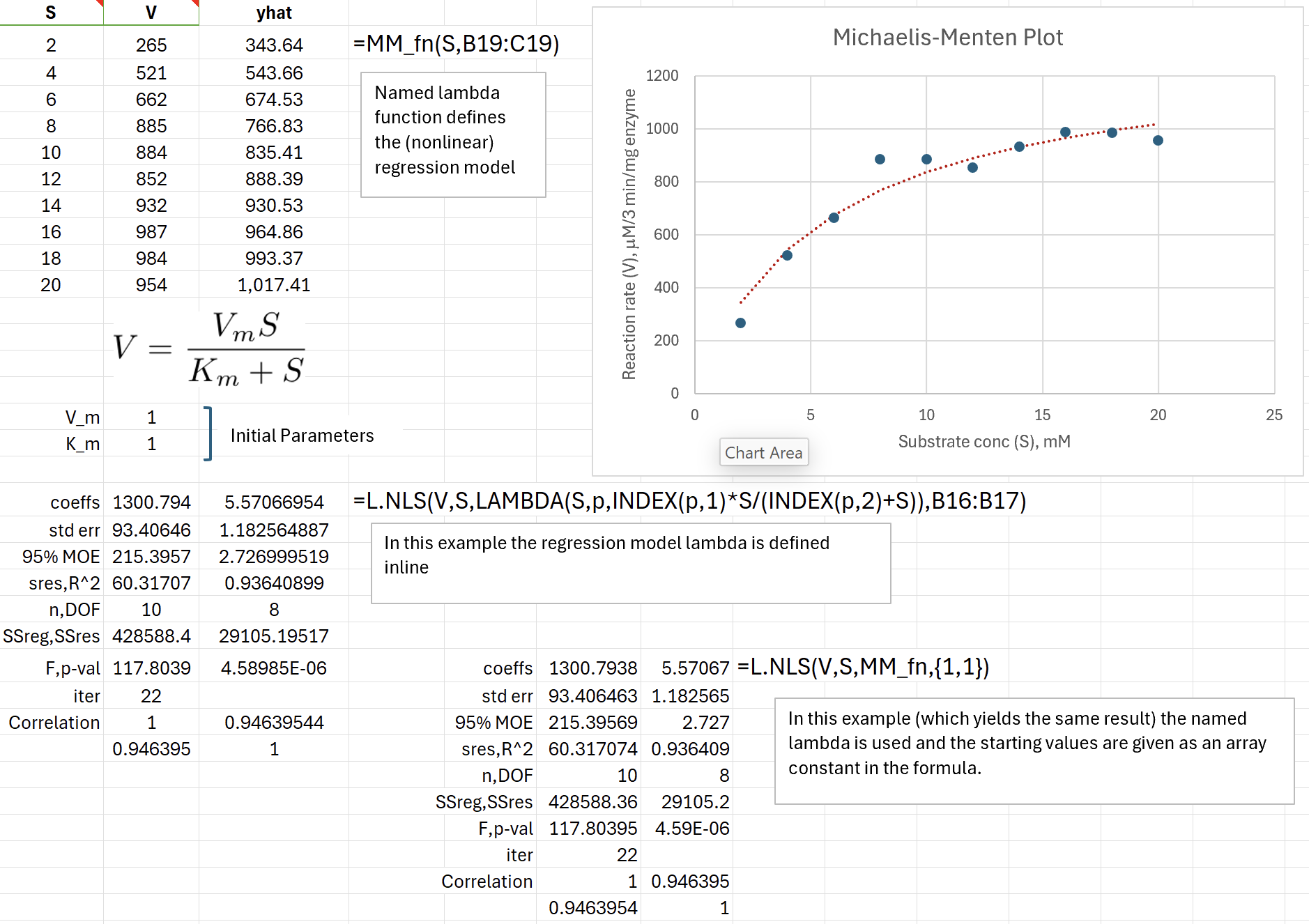
There are two examples of using NLS for nonlinear fitting. In the first example we fit data to the Michaelis-Menten equation, as shown in the image and in the first worksheet of the downloadable Excel file below. There are two calls to NLS shown in the image. One of them defines the lambda inline and references the range of cells containing the initial estimates of the parameters. The other call uses a defined name MM_fn for the same LAMBDA function. That function is also used to calculate the yhat values that were added to the plot.

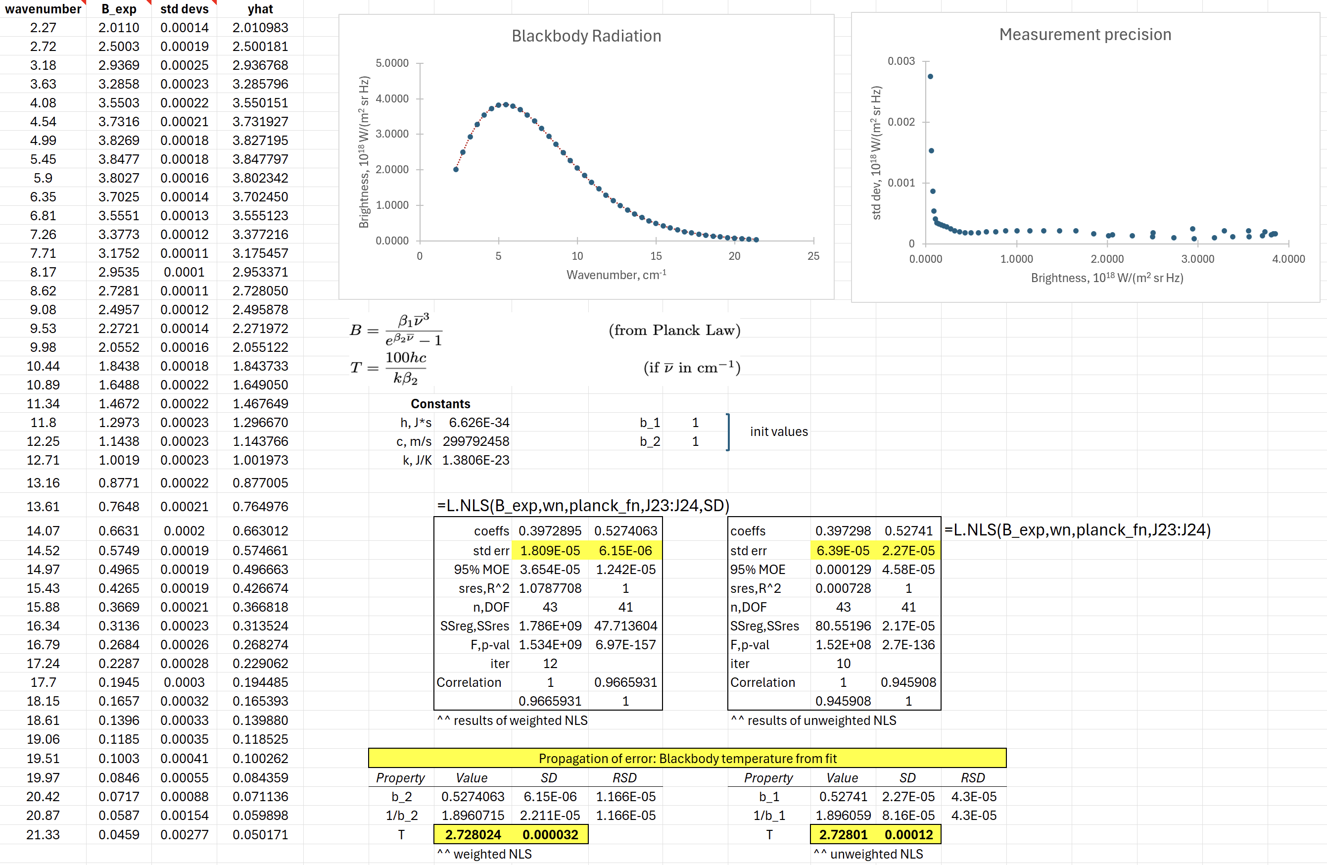
Michaelis-Menten data and fit; NLS with an inline lambda and with a named lambda give the same result, Vm = 1300.8 and Km = 5.57

The next example is on the second worksheet and illustrates the use of weighted nonlinear LS to fit data to a blackbody radiator. Nonlinear LS regression is needed in order to fit the data to Planck’s Law; weighted LS regression is required to obtain the proper standard errors for use in error propagation.

Blackbody fit with weighted and unweighted NLS; both give T = 2.728 K, but the weighted fit has a much smaller SD (0.000032 vs 0.00012)

Download: NonlinearRegression.xlsx

Source Code

Helpers used: _LMFit, _NumJac

NLS = LAMBDA(
    Y, // dependent values as a column vector
    X, // independent values, can be multiple columns
    fn, // LAMBDA(x, p) returning the fitted values as a column
    p0, // starting values of the parameters, row or column
    [S], // optional std devs of the Y values, as a column vector
    [tol], // convergence tolerance (default 1E-8)
    [maxiter], // maximum number of iterations (default 200)
    LET(
        tol, IF(ISOMITTED(tol), 10 ^ -8, tol),
        maxiter, IF(ISOMITTED(maxiter), 200, maxiter),
        S, IF(ISOMITTED(S), 1 + 0 * Y, S),
        // get indices of valid rows for X, Y and S inputs
        Xind, BYROW(X, LAMBDA(X, PRODUCT(--ISNUMBER(X)))),
        NumFilter, Xind * ISNUMBER(Y) * ISNUMBER(S),
        // only keep valid rows
        Xn, FILTER(X, NumFilter),
        Yn, FILTER(Y, NumFilter),
        Sn, FILTER(S, NumFilter),
        n, ROWS(Yn),
        pstart, TOCOL(p0),
        k, ROWS(pstart),
        sw, 1 / Sn,
        wt, sw ^ 2,
        // fn as a function of a parameter column, weighted; #N/A if it
        // errors or doesn't return an n x 1 column
        isRow, COLUMNS(p0) > 1,
        fw, LAMBDA(pc,
            LET(
                v, fn(Xn, IF(isRow, TOROW(pc), pc)),
                IF(IFERROR(AND(ROWS(v) = n, COLUMNS(v) = 1, ISNUMBER(SUM(v))), FALSE), sw * v, NA())
            )
        ),
        fit, _LMFit(fw, pstart, sw * Yn, tol, maxiter),
        p, TAKE(fit, k),
        SSres, INDEX(fit, k + 2),
        // covariance at the estimates, from the column-scaled J'WJ
        J, _NumJac(fw, p),
        Dg, TOCOL(BYCOL(J ^ 2, LAMBDA(c_, SUM(c_)))),
        D, IF(Dg > 0, SQRT(Dg), 1),
        AsInv, MINVERSE(MMULT(TRANSPOSE(J), J) / MMULT(D, TRANSPOSE(D))),
        // variance inflation factors; a redundant parameter gives ~1E15
        vif, INDEX(AsInv, SEQUENCE(k), SEQUENCE(k)),
        singular, IFERROR(OR(MAX(vif) > 10 ^ 12, MIN(vif) <= 0), TRUE),
        DOF, n - k,
        sres, SQRT(SSres / DOF),
        Cov, AsInv / MMULT(D, TRANSPOSE(D)) * sres ^ 2,
        stderrs, TOROW(SQRT(INDEX(Cov, SEQUENCE(k), SEQUENCE(k)))),
        MOE, stderrs * T.INV.2T(5%, DOF),
        yhat, fw(p) / sw,
        SSreg, IF(k > 1, SUM(wt * (yhat - SUM(wt * yhat) / SUM(wt)) ^ 2), SUM(wt * yhat ^ 2)),
        df_num, IF(k > 1, k - 1, 1),
        Rsqr, SSreg / (SSreg + SSres),
        Fobs, SSreg / df_num / sres ^ 2,
        pval, F.DIST.RT(Fobs, df_num, DOF),
        Corr, Cov / MMULT(TOCOL(stderrs), stderrs),
        labels, {
            "coeffs";
            "std err";
            "95% MOE";
            "sres,R^2";
            "n,DOF";
            "SSreg,SSres";
            "F,p-val";
            "iter";
            "Correlation"
        },
        output, IFERROR(
            VSTACK(
                TOROW(p),
                stderrs,
                MOE,
                HSTACK(sres, Rsqr),
                HSTACK(n, DOF),
                HSTACK(SSreg, SSres),
                HSTACK(Fobs, pval),
                INDEX(fit, k + 4),
                Corr
            ),
            ""
        ),
        IF(
            OR(Sn <= 0),
            "ERROR: std devs must be positive",
            IF(
                n <= k,
                "ERROR: need more data points than parameters",
                IF(
                    NOT(ISNUMBER(SUM(fw(pstart)))),
                    "ERROR: fn must return a single column of numbers, one per data point, at p0",
                    IF(
                        OR(INDEX(fit, k + 5) = 1, NOT(ISNUMBER(SUM(J)))),
                        "ERROR: fn failed near the current estimates; try other starting values",
                        IF(
                            AND(INDEX(fit, k + 3) <> 1),
                            "ERROR: did not converge in " & maxiter & " iterations; try other starting values or a larger maxiter",
                            IF(
                                singular,
                                "ERROR: the parameters can't all be estimated (one has no effect, or two are redundant); try other starting values",
                                IFERROR(HSTACK(labels, output), "")
                            )
                        )
                    )
                )
            )
        )
    )
);

WLS Sres