MCM_error(_V)

Description

The MCM_error functions (ie, MCM_error and MCM_error_V) use the Monte Carlo method to analyze the propagation of uncertainty due to the transformation of random variables. The first function is non-volatile and seedable; the second function is volatile, faster, and has a better RNG.

Syntax

The syntax is the same as MCM and MCM_V; documentation of those functions should be consulted for details. To summarize:

• MCM_error(vars, se_vars, fn, [N=1000], [DFs], [skew=0], [kurt], [seed_str])
• MCM_error_V(vars, se_vars, fn, [N=1000], [DFs], [skew=0], [kurt])

Both functions return $3 + k$ values in the output (where $k$ is the number of variables). Of course the _V version is volatile. The values are:

• The point estimate of the transformed variables.
• The bias introduced by the transformation. This is not the same thing as propagation of bias. This is the bias due to any skewness introduced by the transformation itself. Such skewness would pull the mean of the distribution in one direction or the other. The bias is typically quite a bit less than the random error and so it is often ignored.
• The standard error of the simulated values. This is the prediction of the MC method for the standard deviation, the value directly comparable to the prediction of the linear error propagation method.
• Contributions (one for each of the variables) towards the total variance. This is the one-at-a-time (OAT) contribution assessed by only allowing one of the variables to have uncertainty while the others are fixed at their mean values. The variance introduced by a given variable is divided by the variance when all are allowed to vary. They may not sum to 100% because of the randomness of simulations but also because the OAT method does not account for higher-order interactions between variables.

Example

We will continue to use the same example as with MCM and MCM_CI. The example below compares the MC method with the linear approximation method that is based on partial derivatives (ie, first-order Taylor expansion). The ability of the MCM methods to include the effects of skew is demonstrated in this example.

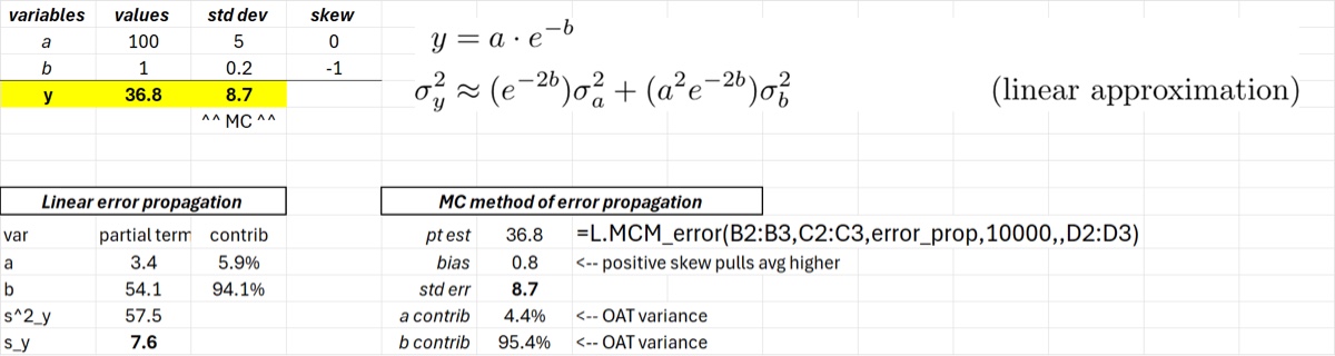
This example is set up in the attached Excel file. You should open it up and try looking at the effects of increasing error, changing skew, or degrees of freedom.

Download: MCM-error.xlsx

Source Code

Helpers used: FSolve, FSolveBump, FSolveLadder, FSolveMonotonic

The source code for the nonvolatile sibling MCM_error is shown below. The code for MCM_error_V is identical except it calls MCM_V (without a seed) on line 9.

MCM_error = LAMBDA(
    vars, se_vars, fn,
    [N], [DFs], [skew], [kurt], [seed_str],
    LET(
        N, IF(ISOMITTED(N), 1000, N),
        varsRow, TOROW(vars),
        seRow, TOROW(se_vars),
        k, COLUMNS(varsRow),
        sims, MCM(vars, se_vars, fn, N, DFs, skew, kurt, seed_str),
        IF(
            ISTEXT(INDEX(sims,1,1)),
            sims,
            LET(
                trueValue, fn(varsRow),
                bias, AVERAGE(sims) - trueValue,
                stderrVal, STDEV.S(sims),
                totalVar, VAR.S(sims),
                oatFractions, MAP(
                    SEQUENCE(1,k),
                    LAMBDA(j,
                        LET(
                            isolatedSE, IF(SEQUENCE(1,k) = j, seRow, 0),
                            isolatedSims, MCM(vars, isolatedSE, fn, N, DFs, skew, kurt, seed_str),
                            VAR.S(isolatedSims) / totalVar
                        )
                    )
                ),
                VSTACK(trueValue, bias, stderrVal, TOCOL(oatFractions))
            )
        )
    )
);