KDEmax

Description

KDEmax returns the value that corresponds to the maximum density of data as estimated by the kernel density estimate. This value, called the kernel mode estimator (KME), is a robust, distribution-agnostic location statistic.

Syntax

KDEmax(data, [bw=1], [points=75], [start=min], [end=max]) where

• data is the input univariate data (any shape)
• bw is the smoothness scaling factor relative to the Silverman rule-of-thumb bandwidth
• points is the number of grid points over the range used in the first-stage (“coarse”) search for the maximum (see Source Code section for details)
• start and end define the range over which the search for the KME occurs; by default this is the entire range of the data

The function returns a single locator statistic, the KME. It is the value around which the input data is most densely clustered. It should be viewed as a robust locator statistic, similar to the median and the trimmed mean.

Example: KDEmax as a robust locator statistic

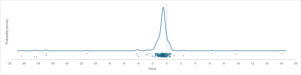
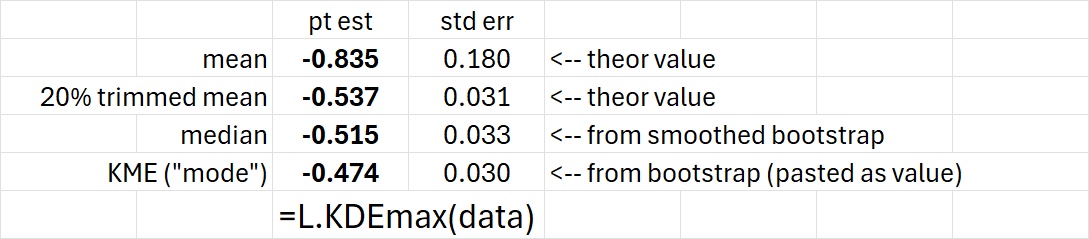
An example of how the KDEmax might be useful is shown in the screenshots below, and in the first sheet of the Excel file attached below. The data has a significant negative skew which pulls the mean to a significantly more negative value than the bulk of the data. The other three location estimators are all more robust and have about the same standard error. The KDEmax is estimating the mode using the maximum of the KDE shown in the plot, and the ordering of mean < median < mode occurs as expected for data with a negative skew.

Download: KDEmax.xlsx

Edge Cases and Bandwidth Choice

There are two situations where KDEmax may return a flawed estimate of the mode:

• when the mode is near a boundary condition
• when there is a sharp peak (large local curvature at the max) in a skewed distribution

Both conditions can be alleviated somewhat, though not completely eliminated, by choosing smaller bandwidths than the default.

Let us consider the case of the standard lognormal distribution, where both of the above situations apply. The theoretical distribution and the KDE with the default bandwidth bw=1 are shown below. The offset between the max of the KDE for this sample (which is what KDEmax returns) and the true mode is obvious, and is not specific to this draw.

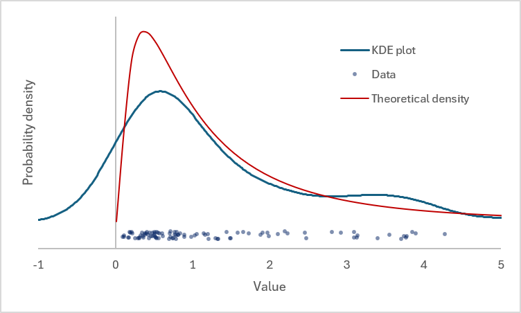
This plot is shown on the second worksheet of the Excel file attached earlier. Using smaller bandwidths helps but does not completely erase the bias. The plot below shows the effect of changing bw for this specific sample (the mode of the standard lognormal distribution is $\frac{1}{e} = 0.368$).

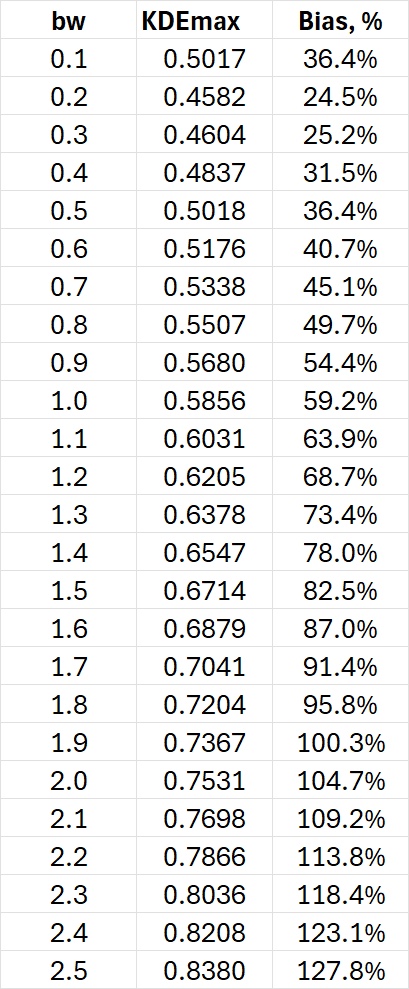
In this case there are two contributions to the bias, and simulations with the lognormal show that they contribute roughly equally:

• the KDE does not estimate the probability density well near a boundary
• the mode in the standard lognormal is fairly sharp and, when combined with skewness, this leads to increasing bias at higher bandwidths.

So why not set the default to a lower bandwidth? The following example illustrates the trade-offs involved in choosing a too-low bandwidth. We illustrate with a chi-squared distribution with 25 degrees of freedom: the skew is relatively modest and the mode is known to be $\nu-2 = 23$. The figure below compares the theoretical distribution with the KDE of a 100-sample draw from the population.

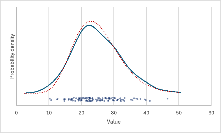
Seems like a reasonable fit; there are no boundary concerns here. The following are simulations (1000 loops with draws of 100 each) that show the effect of the bandwidth on both bias and the standard error of the KDEmax.

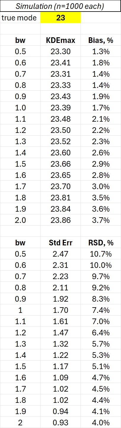
These numbers are all in the third worksheet in the XL file attached earlier. You can see that there is a trade-off with skewed distributions:

• larger bandwidths pull the KDEmax value towards the mean (ie in the direction of the skew), increasing the bias
• larger bandwidths decrease the standard error of the KDEmax estimate, improving efficiency.

Thus there is a trade-off between accuracy and precision. The default bandwidth of bw=1 seems a reasonable compromise.

But there is only bias in the KDEmax value when the distribution is skewed. What about symmetric distributions? Shouldn’t we then choose a much larger bandwidth since we don’t have to worry about bias?

The problem is a hidden third factor: larger bandwidths make the statistic less robust to outliers. The above simulations had no outliers and so didn’t show this effect. For distributions that are prone to outliers (ie with long tails) you don’t want the bandwidth to be too large. One of the main reasons to use the KDEmax as a locator statistic instead of the mean is that you want some robustness, and if you choose a very large bandwidth then the KDEmax simply becomes an overcomplicated way of estimating the mean.

The bottom line: the default value of bw = 1 is a good compromise between bias, efficiency, and robustness for many situations, but you should definitely explore the effects of changing the bandwidth for your situation. Bootstrapping the KDEmax is one way to investigate this for a specific sample; see the Bootstrap and related functions for more details.

Source Code

Searching for the KME is computationally expensive, particularly if combined with bootstrapping. To reduce the load, the search is divided into two parts:

• a coarse search to identify the location of the global max
• a finer search to identify that max

The points argument determines the coarseness of that initial search; the default value of 75 was obtained through simulations of sample sizes below $n = 500$. The default bandwidth scaling of 1 was likewise determined through simulations to be a good compromise between bias and efficiency (ie, standard error). The larger bandwidths that have been promoted lately in the literature were found to result in unacceptably large bias.

But for sample sizes above 500 you might want to adjust the defaults to avoid the risk of finding a local maximum instead of the global maximum. Possible strategies to do so while minimizing computational costs:

• reducing the range (so that the sample size in the range is 500 or smaller)
• increasing the number of points so that the initial search is not too coarse
• increasing the bandwidth

Highly skewed data can also result in incorrect results; in that situation you might want to try different function parameters to see what works best.

KDEmax = LAMBDA(
    X, // input data (any shape)
    [bw], // smoothing bandwidth factor (see KDE function); default 1
    [points], // points in the coarse localization pass; default 75
    [start],
    [end], // start and end values of the coarse localization range (default MIN(X)/MAX(X))
    LET(
        bw, IF(ISOMITTED(bw), 1, bw),
        points, IF(ISOMITTED(points), 75, points),
        start, IF(ISOMITTED(start), MIN(X), start),
        end, IF(ISOMITTED(end), MAX(X), end),
        Xc, TOCOL(X),
        Xn, FILTER(Xc, ISNUMBER(Xc)),
        n, COUNT(Xn),
        H, 1.059 * MIN(STDEV.S(Xn), IQR(Xn, TRUE)) * n ^ (-0.2),
        W, H * bw,
        // coarse pass: locate the right basin
        D, Density(Xn, bw, points, start, end),
        y, INDEX(D, , 2),
        x0, XLOOKUP(MAX(y), y, INDEX(D, , 1)),
        // refine: fixed mean-shift iterations, each moving the estimate to
        // the kernel-weighted mean of the data around its current position
        step, LAMBDA(xhat, _, LET(wts, NORM.S.DIST((xhat - Xn) / W, FALSE), SUMPRODUCT(wts, Xn) / SUM(wts))),
        REDUCE(x0, SEQUENCE(20), step)
    )
);