JitterPlot

Description

JitterPlot returns two columns of values that can be plotted to create a strip plot of data that overlap. It is a fairly limited function meant to visualize univariate data on a number line and generally works best when combined with other plots that visualize distributions, such as histograms, KDE plots, and boxplots.

If you have a grouping variable and want to create jitterplots by group, with different colors or markers, then you have to do so manually by applying the function to data filtered by group and adding them to a plot. (Honestly it is faster to just use Excel’s boxplot functionality in those cases, or to use Python’s matplotlib or seaborn libraries within Excel.)

Syntax

JitterPlot(data, [mean=0], [halfwidth=1]) where

data is the univariate data (any shape; non-numeric values are filtered out)
mean is the mean of the added jitter noise
halfwidth is the maximum jitter in either direction from mean

The function returns two columns of values to be plotted to create the jitterplot. The first column is just a copy of the original data while the second column is the value of mean plus a little noise.

Note that JitterPlot uses another CLS-Stats function, runif, to generate the jitter noise (using a uniform probability distribution). This function is used, instead of Excel’s RANDARRAY function, so that the output of JitterPlot is not volatile. If you wish to reset the seed (changing the jitter) then invoke the Randomize Seed routine in the Analysis item in the CLS-Stats ribbon group.

Example

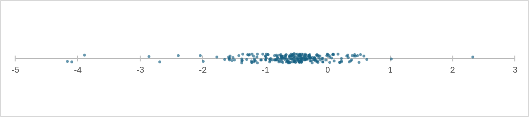
Below is the kind of plot that can be generated from the output of JitterPlot. All of the information is in the X-axis; the jitter along the Y-axis is solely there to be able to view data that are clustered together as semi-distinct points. Adding some transparency to the symbols (as I did below) means that overlapping data will also be indicated by darker colors.

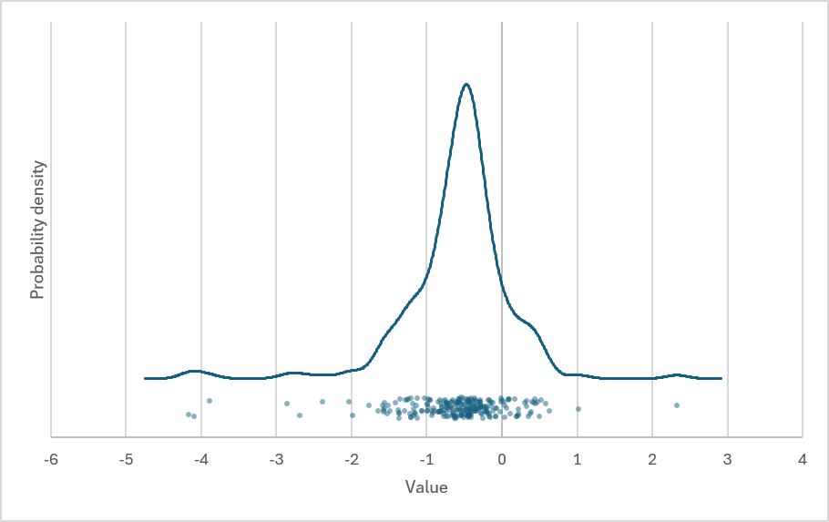
Jitterplot of the data along a value axis from -5 to 3, points clustered between -2 and 1 with a few outliers

As implemented in CLS-Stats, jitterplots are probably best combined with other types of plots that show distribution. An example is shown below, combining the above jitterplot with a KDE plot of the data. Use the mean and halfwidth function arguments to control where the jitterplot is placed on the plot and how much jitter is used.

KDE curve of the data with the jitterplot drawn just beneath it

The Excel file containing both of the above plots (and the function calls that generated them) is attached below.

Download: Jitterplot.xlsx

Source Code

JitterPlot = LAMBDA(
    data, // input data as a column
    [mean], // the mean of the jittered points (default 0)
    [halfwidth], // max vertical jitter in either direction (default 1)
    LET(
        Xc, TOCOL(data),
        Xn, FILTER(Xc, ISNUMBER(Xc)),
        mean, IF(ISOMITTED(mean), 0, mean),
        halfwidth, IF(ISOMITTED(halfwidth), 1, halfwidth),
        // use unique seed to avoid potential noise correlation issues
        HSTACK(Xn, 2 * halfwidth * runif(
            COUNT(Xn),,,,,SetSeed(CLS_SystemSeed & ADDRESS(ROW(),COLUMN()) & "JitterPlot")
        ) + mean - halfwidth)
    )
);

Note that runif is another CLS-Stats function, one that samples a uniform probability distribution (in this case in the range [0,1]). It is used here so that JitterPlot is not volatile.

Density KDE