Density

Description

Density returns the X and Y values for a Kernel Density plot. It defaults to intelligent values for the range and number of X values but these can be overridden in the function call. The user can also choose the width of the kernel, controlling the amount of smoothing.

Syntax

Density(data, [bw=1], [points=1000], [start], [end])

• data is the input data to be smoothed
• bw is the smoothing factor relative to the Silverman rule of thumb: a value of 1 (the default) is generally acceptable for unimodal data
• points is the number of KDE values to calculate
• start and end set the range of X values over which to calculate the KDE

When exploring data it is a good idea to try a number of different smoothing factors and choose the one that suits your needs. If the default range of X values is too wide, or includes values that are physically impossible, then you can substitute other values in the function call.

Example

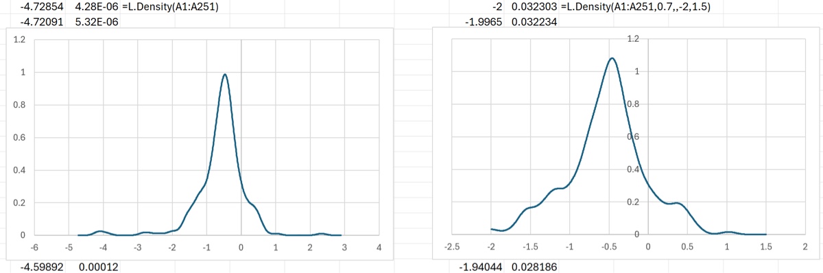
The screenshot below shows how to call the function with the defaults as well as the effects of changing those defaults. The XL spreadsheet is also given below.

Download: Density.xlsx

KDE at Boundaries

The (uncorrected) KDE has known issues near boundaries. To illustrate, consider the figure below which compares the KDE of 100 data points drawn from a standard lognormal distribution to the theoretical distribution.

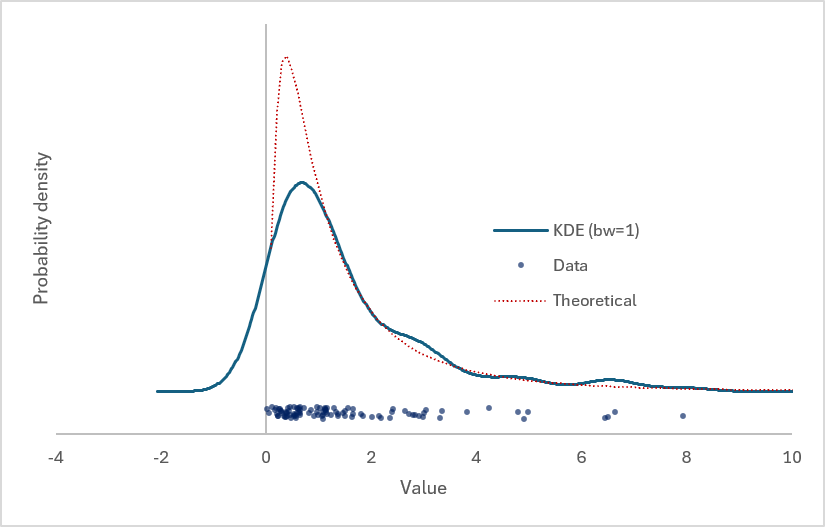
Negative values are not allowed in the lognormal distribution; this distribution is used to describe a number of natural phenomena such as the distribution of pollutant concentrations in groundwater wells, so the above case has practical import.

The KDE when called with the default bandwidth bw = 1 does not accurately describe the probability density near the boundary. It fails in three respects:

• it incorrectly shows a nonzero probability of negative values
• it underestimates the probability density of the positive values near the boundary
• the mode of the KDE is shifted relative to the mode of the actual distribution.

These problems can be lessened somewhat by choosing a smaller bandwidth, at the expense of a noisier KDE. The figure below shows the same comparison but with bw = 0.5.

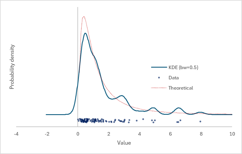
There are a number of methods to correct the KDE (eg, using asymmetric kernel functions) but these are not implemented here. For more accurate estimation of the probability density near the boundary, a histogram might be preferable.

Source Code

Density = LAMBDA(
    X, // input data (any shape)
    [bw], // smoothing bandwidth factor (see KDE function); defaults to 1
    [points], // number of points at which KDE is evaluated (defaults to 1000)
    [start],
    [end], // first and last X values at which to evaluate the KDE (see code below for defaults)
    LET(
        // convert tables & rows to a column
        Xc, TOCOL(X),
        // now filter for numeric values
        Xn, FILTER(Xc,ISNUMBER(Xc)),
        // default values bw=1, points=1000
        bw, IF(ISOMITTED(bw), 1, bw),
        points, IF(ISOMITTED(points), 1000, points),
        n, COUNT(Xn),
        // calculate window width W
        s, MIN(STDEV.S(Xn), (QUARTILE.INC(Xn,3)-QUARTILE.INC(Xn,1))/1.34897950039216),
        H, 1.059 * s * n ^ (-0.2), // rule-of-thumb BW times the scaling factor bw
        W, H * bw,
        // set the default start and end values if omitted
        // defaults are 3 bandwidths above and below the max and min values, respectively
        start, IF(ISOMITTED(start), MIN(Xn) - 4 * H, start),
        end, IF(ISOMITTED(end), MAX(Xn) + 4 * H, end),
        // create the x-values at which to evaluate the KDE
        xi, SEQUENCE(points, 1, start, (end - start) / (points - 1)),
        // now calculate the KDE vector and return the two columns
        k, BYROW(xi, LAMBDA(val, SUM(NORM.S.DIST((val - Xn) / W, FALSE)))),
        HSTACK(xi, k/(n*W))
    )
);