BootCompare

Description

BootCompare returns a bootstrapped comparison statistic for two independent samples. Imagine you want to compare the medians of two independent samples, A and B. The process for a bootstrap-based comparison would go like this:

1. Obtain a bootstrap sample of each sample.
2. Calculate the difference in medians of those samples.
3. Repeat another $B-1$ times and output the result.

The result is $B$ values of the bootstrapped comparison. The user is free to create whatever comparison statistic they wish, such as the log of the ratio of MAD values.

Syntax

The function is basically the two-sample version of Bootstrap and shares a similar syntax, with the addition of a second sample:

BootCompare(sample1, sample2, fn, [B=1000], [bw=0]), where

• sample1 and sample2 are the samples whose properties the user wishes to compare. The samples are either univariate (row or column vectors) or multivariate (matrix, with rows as observations). Resampling of matrices is by rows.
• fn is a LAMBDA callback function that returns a comparison statistic calculated from two statistics, one for each sample. The function must take two parameters and return a scalar value: the bootstrapped statistic. For example, to compare the means one would use LAMBDA(x, y, AVERAGE(x) - AVERAGE(y)).
• B is the number of bootstraps to run; the default is 1000
• bw is the bandwidth of a smoothed bootstrap; the default is no smoothing. The argument is ignored if sample1 and sample2 are multivariate. The value has the same meaning as in the KDE functions (such as Density). Smoothing is applied to each bootstrap sample, before the comparison statistic is calculated. In other words, if one used

// comparison of medians of two samples
=BootCompare(sample1, sample2, LAMBDA(x, y, MEDIAN(x) - MEDIAN(y)), 1000, 1)

then each bootstrap comparison statistic is the difference between two smoothed medians.

Like all the bootstrap functions, BootCompare is volatile since it is based on BootSample, which uses Excel’s RANDARRAY.

Example

Below is a bootstrapped comparison of median measurement errors, male vs female, using a smoothed bootstrap with BootCompare. The boxplots of the errors show the presence of many outliers while BootCompare allows the examination of the distribution of the comparison statistic, as below with the QQ plot against the standard normal distribution.

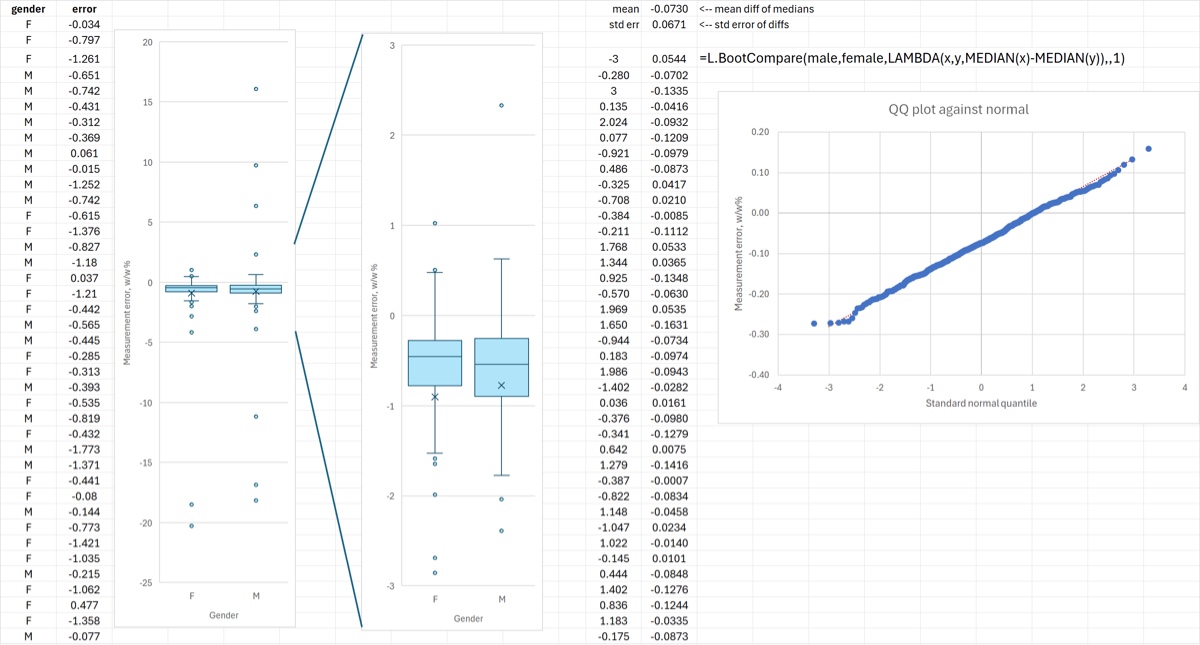
The Excel file is below. Since BootCompare is volatile, the numbers you see won’t be exactly the same. Boost the number of bootstraps for less sampling variability.

Download: BootCompare.xlsx

Source Code

Helpers used: BootObs

BootCompare = LAMBDA(
    sample1, sample2,   // two independent samples to compare
    fn,                 // lambda function returns a comparison stat
    [B],                // number of bootstrap sample comparisons to return
    [bw],               // smoothing bandwidth factor, same meaning as KDE's bw (default 0, unsmoothed)
    LET(
        B, IF(ISOMITTED(B), 1000, B),
        bw, IF(ISOMITTED(bw), 0, bw),
        MAP(
            SEQUENCE(B),
            LAMBDA(
                _,
                fn(
                    BootSample(sample1, bw),
                    BootSample(sample2, bw)
                )
            )
        )
    )
);