BinomialTest

Description

BinomialTest performs a binomial test, a nonparametric alternative to a one-sample t-test or a paired t-test. It returns the p-value of the test.

Syntax

BinomialTest(data1, data2, [Ha = 2]) where

• data1: the first group of observations (any shape)
• data2: either a single value (one-sample test) or data the same size as data1 (paired test)
• Ha: specifies the nature of the alternative hypothesis. If Ha = 2 (the default) then a two-tailed test is performed. If Ha = 0 then test if data1 < data2. If Ha = 1 then test if data1 > data2.

The output is the scalar p-value. If you prefer to perform hypothesis testing using a confidence interval, use the BinomialCI function.

Example

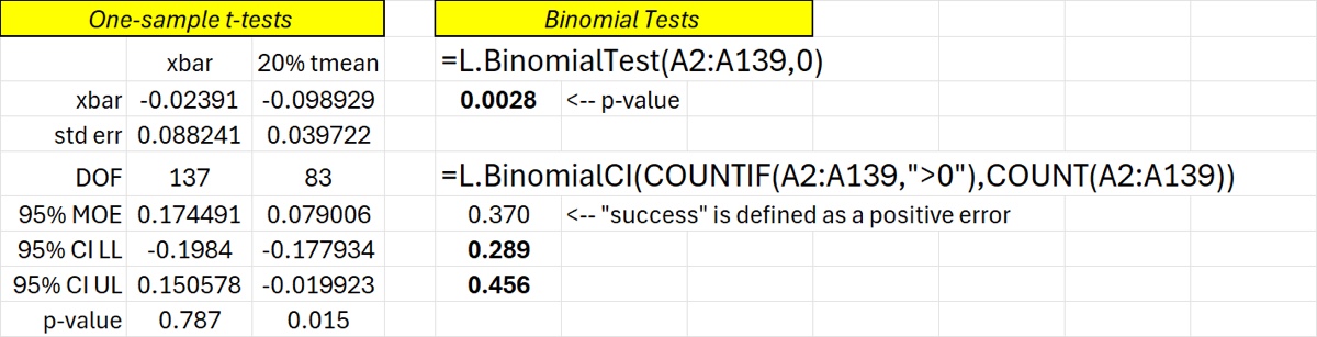
In the example below, 138 students performed measurements and the question is whether those measurements are biased (in either direction); this is real data by the way. The standard method is to use a one-sample t-test, comparing the resulting mean to zero (or, equivalently, ascertaining if the confidence interval contains zero). The problem is that there are some significant outliers in the data. The untrimmed mean fails to show any bias while the 20% trimmed mean demonstrates a bias of around 0.1 w/w% that is (barely) statistically significant.

But if one observes that nearly two-thirds (63%) of the errors are negative one might wonder what a binomial test would have to say. The binomial test is predicated on the notion that a given error should be equally likely to be positive or negative if no measurement bias is present. In this example, the BinomialTest function returns a p-value of 0.003 which is well below a typical significance level; this test seems to have more statistical power for this particular sample.

p-values are still used but have fallen out of favor somewhat; confidence intervals give the same conclusion and give more information about the magnitude of the effect. The BinomialCI function returns a confidence interval for the proportion of “successes”, however that is defined. In this example we define “success” as a positive error and the output of BinomialCI shows us the magnitude of the effect (37% of the errors are positive) and quantifies the uncertainty as a 95% confidence interval: the true probability of producing a positive error is between 29% and 46%, with 95% confidence. Since that CI does not contain 50% we are free to reject the null hypothesis and conclude that the procedure is biased, with a predilection for underestimating the value. (The advantage of the 20% trimmed mean t-test is that it gives us a sense of the magnitude of that bias.)

Download: BinomialTest.xlsx

Source Code

BinomialTest = LAMBDA(
    data1, // first data set, any shape
    data2, // either a single value or data same size as data1
    [Ha], // options for alternative hypothesis
    // If Ha=2 (default) then a 2-tailed test is performed.
    // If Ha=0 then test if data1<data2
    // If Ha=1 then test if data1>data2
    LET(
        Ha, IF(ISOMITTED(Ha), 2, Ha),
        n_1, COUNT(data1),
        n_2, COUNT(data2),
        // exclude ties from analysis
        x_1, FILTER(data1, data1 <> data2),
        x_2, IF(n_2 = n_1, FILTER(data2, data1 <> data2), data2),
        N, COUNT(x_1),
        // calculate p-hat
        Ns, IF( // number of successes
            Ha = 0,
            SUM(--(x_1 < x_2)),
            SUM(--(x_1 > x_2)) // for 2-tailed test doesn't matter which tail
        ),
        p_hat, Ns / COUNT(x_1),
        p_val, IFS(
            p_hat = 0.5,
            1,
            OR(Ha = 0, Ha = 1),
            1 - BINOM.DIST(MAX(Ns - 1, 0), N, 0.5, TRUE),
            Ha = 2,
            LET(
                limits, IF(
                    p_hat > 0.5,
                    VSTACK(N - Ns + 1, Ns - 1), // right side of distr
                    VSTACK(Ns + 1, N - Ns - 1) // left side
                ),
                1 - BINOM.DIST.RANGE(N, 0.5, MAX(INDEX(limits, 1), 0), MIN(INDEX(limits, 2), N))
            )
        ),
        p_val
    )
);