ANOVA

Description

ANOVA performs analysis of variance of the input data; currently it accepts a single explanatory (grouping) factor – it performs 1-factor ANOVA. There are two lambda functions that do this in the CLS-Stats library: ANOVA and ANOVA1S. They differ only in the format of the inputs.

ANOVA will be the more commonly used of the two functions: it accepts the input arguments as two column vectors, similar to regression functions, which is fitting since ANOVA can be viewed as a form of regression in which the explanatory variables are categorical instead of numeric.

Syntax

ANOVA(Y, X, [sb_stats]) where

Y is a column vector of numeric/response variables and
X is a column vector of categorical variables
sb_stats is an optional boolean (default FALSE) on whether to display an additional column with information about the $s_b$ estimate of between-group standard deviation $\sigma_b$ .

The two inputs must have the same number of rows. If either has an empty cell then both entries in that row will be filtered out of the data before the calculations. This allows the user to explore the effects of removal of individual observations (eg outliers) on the calculation.

ANOVA is an analysis of how much of the variability in the observed Y variable (numeric observations or measurements) is explained by group membership as described by the X variable (categorical variables). Note that if the X values are numbers they are still treated in the ANOVA calculations as labels without magnitude.

The default output of the function is a labeled ANOVA table with four rows and four columns (without counting the labels), as outlined below.

	SS	DF	MS	s
Within
Between
Total
F test

The first three rows are distinct from the last row. The entries of the first three rows, described below, partition the total variability between that explained by group membership (the $X$ variable) and the residual variability within each group (eg, measurement noise).

SS are the three Sum of Squares terms: within-group $SS_W$ , between-group $SS_B$ , and the total $SS_T$ . Sums of squares are the sum of squared deviations from the mean and are a measure of unscaled variability. They are related as $SS_T = SS_B + SS_W$
DF are the degrees of freedom for each SS term. They too are related as $DF_T = DF_B + DF_W$ .
MS are the mean sums of squares, $MS = \frac{SS}{DF}$ . They are scaled measures of variability (ie, variances).
The fourth column contains standard deviation terms.
- $s_W$ is the within-group standard deviation, an assessment of the reproducibility of repeated observations/measurements within a given group. It is simply the square root of the $MS_W$ term; it is also called the pooled standard deviation.
- $s_B$ is the between-group standard deviation, an assessment of the contribution of group membership to the overall variability, independent of the variability within a group.
  $\begin{align*} s_b &= \sqrt{\dfrac{MS_B - MS_W}{n_0}}\\ n_0 &= \frac{1}{k-1} \left( {\sum n_i - \dfrac{\sum n_i^2}{\sum n_i}} \right) \end{align*}$
  where $n_0$ is the weighted-average group size, $n_i$ is the number of observations in group $i$ , and $k$ is the number of groups. If all groups have the same number of measurements ( $n$ ) then $n_0$ reduces to $n$ . Note that if $MS_B < MS_W$ then $s_b$ is reported as 0.
- $s_T = \sqrt{s_B^2 + s_W^2}$ describes the variability of any given value in $Y$ as the sum of its contributions (group membership + residual)

The very last row is for hypothesis testing (“is group membership a statistically significant source of variability?”) and is not connected to the column labels.

The first entry is the test statistic. It is the ratio of between-group and within-group mean squared values, $F_\text{obs} = \frac{MS_B}{MS_W}$ . If the within-group observations are normally distributed then the test statistic follows an $F$ -distribution. The question that the hypothesis test is addressing is, is this value significantly greater than one, $F_\text{obs} \overset{?}{>} 1$ .
The second entry is the (parametric) lower confidence bound for the test statistic; in other words, the true ratio of mean squares is larger than this number with 95% confidence. Hypothesis testing with ANOVA is usually a one-tailed test, which is why a lower bound is supplied rather than two boundaries of a confidence interval. If one prefers to report confidence intervals instead of p-values, then this is the value to report. It gives the lower bound for the quantity $(n_0 \sigma_B^2 + \sigma_W^2) / \sigma_W^2$ .
The third entry is the critical value $F_\text{crit}$ of the test statistic, assuming that statistic follows an $F$ -distribution. If the test statistic is larger than this value then group membership is “proven” with 95% confidence. Another way of thinking of this value: it is the minimum value at which we can say (with 95% confidence) that the fact that the test statistic is greater than one is due to an underlying contribution of group membership rather than random variation.
The last entry is the p-value of the hypothesis test. If it is less than the desired significance level then group membership is “proven” to be statistically significant.

If you set sb_stats = TRUE then two columns are added to the output: the first, labeled s_b, contains three additional items, and the second contains labels for them.

The first is the degrees of freedom $\nu$ of the estimate $s_b$ , calculated with the Satterthwaite equation for a difference of MS values:
$\nu \approx \frac{(MS_B - MS_W)^2}{MS_B^2 / \nu_B + MS_W^2 / \nu_W}$
The next two terms are the lower and upper bounds of the 95% confidence interval calculated using a chi-squared distribution (but see note in the Source Code section below)
It is worth noting that $\sigma_B$ is quite poorly determined in some circumstances (when $\text{MS}_B \approx \text{MS}_W$ for example). If $\text{MS}_B \le \text{MS}_W$ then $s_b$ is reported as zero, the lower bound as zero, and the degrees of freedom and upper bound as “n/a”.

Example

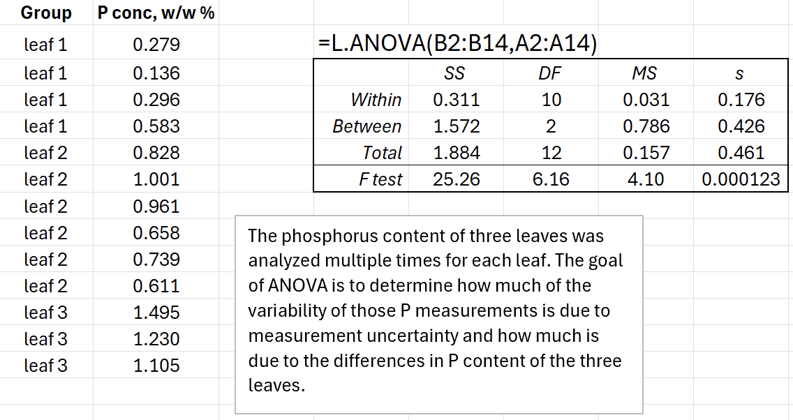
An example is given below; the Excel file is also attached. The question here is whether there are different levels of phosphorus in each of the leaves and, if so, how much of the variability of the observations is due to that fact compared to the inherent uncertainty of the measurement process. The answer to the question, “do the leaves have different P concentrations?”, is addressed by the hypothesis test statistics in the last row. The answer to the question, “what is the magnitude of the leaf-to-leaf variability in P content and how does it compare to the measurement uncertainty?” is answered by the first three entries in the last column.

ANOVA of phosphorus content in three leaves: data and the ANOVA table, F = 25.26 with p = 0.000123

Download: ANOVA.xlsx

Source Code

Note that if sb_stats = TRUE then GAMMA.INV is used to find the CI bounds since it accepts non-integer degrees of freedom (which is certainly the case here for $s_b$ ) with GAMMA.INV(p, df/2, 2) being used in lieu of CHISQ.INV(p, df).

ANOVA = LAMBDA(
    Y, // column vector of data
    X, // column vector of groups (same length as Y)
    [sb_stats], // add columns of s_b info? (default FALSE)
    LET(
        sb_stats, IF(ISOMITTED(sb_stats), FALSE, sb_stats),
        // eliminate blanks from either vector
        Xb, FILTER(X, NOT(ISBLANK(X)) * NOT(ISBLANK(Y))),
        Yb, FILTER(Y, NOT(ISBLANK(X)) * NOT(ISBLANK(Y))),
        groups, UNIQUE(Xb),
        /*
         For some reason COUNTIF and AVERAGEIF in the lines below only work if
         the inputs are ranges rather than (say) the result of a FILTER operation.
         Using BYROW fixes the problem.
        */
        // n_i, COUNTIF(X, groups),
        // xbar_i, AVERAGEIF(X, groups, Y),
        n_i,    BYROW(groups, LAMBDA(grp, SUM(--(grp = Xb)))),
        xbar_i, BYROW(groups, LAMBDA(grp, AVERAGE(FILTER(Yb, Xb = grp)))),
        s_i,    BYROW(groups, LAMBDA(group_i, STDEV.S(FILTER(Yb, Xb = group_i)))),
        xbar_global, AVERAGE(Yb),
        SS_b, SUM(n_i * (xbar_i - xbar_global) ^ 2),
        // need to avoid using groups with just one member in calculating SS_w
        SS_w, SUM(FILTER(n_i - 1, n_i > 1) * FILTER(s_i ^ 2, n_i > 1)),
        SS_t, DEVSQ(Yb),
        DF_b, COUNTA(groups) - 1,
        DF_w, SUM(n_i - 1),
        DF_t, COUNT(Yb) - 1,
        MS_b, SS_b / DF_b,
        MS_w, SS_w / DF_w,
        MS_t, SS_t / DF_t,
        s_w,  SQRT(MS_w),
        n0,   (SUM(n_i) - SUMSQ(n_i) / SUM(n_i)) / (COUNTA(groups) - 1),
        // if MS_b < MS_w then s_b is not defined; output zero in that case
        s_b,  IFERROR(SQRT((MS_b - MS_w) / n0), 0),
        s_r,  SQRT(s_w ^ 2 + s_b ^ 2),
        // last row entries: hypothesis testing
        Fobs,   MS_b / MS_w,
        F_LL,   Fobs / F.INV.RT(5%, DF_b, DF_w),
        F_crit, F.INV.RT(5%, DF_b, DF_w),
        P_obs,  F.DIST.RT(Fobs, DF_b, DF_w),
        results, VSTACK(
                HSTACK("",        "SS",   "DF",   "MS",   "s"),
                HSTACK("Within",  SS_w,   DF_w,   MS_w,   s_w),
                HSTACK("Between", SS_b,   DF_b,   MS_b,   s_b),
                HSTACK("Total",   SS_t,   DF_t,   MS_t,   s_r),
                HSTACK("F test",  Fobs,   F_LL,   F_crit, P_obs)
            ),
        // optional columns of s_b info, with their own IFERROR so a
        // problem here can't wipe out the ANOVA table itself
        sb_col, IFERROR(
            IF(
                MS_b > MS_w,
                LET(
                    // Satterthwaite DOF for s_b^2 = (MS_b - MS_w)/n0 (a difference)
                    DF_sb, (MS_b - MS_w) ^ 2 / (MS_b ^ 2 / DF_b + MS_w ^ 2 / DF_w),
                    // GAMMA.INV = chi-square quantile that allows fractional DOF
                    // (CHISQ.INV truncates DOF to an integer)
                    LL, SQRT(DF_sb * s_b ^ 2 / GAMMA.INV(0.975, DF_sb / 2, 2)),
                    UL, SQRT(DF_sb * s_b ^ 2 / GAMMA.INV(0.025, DF_sb / 2, 2)),
                    VSTACK("s_b", DF_sb, LL, UL, "")
                ),
                VSTACK("s_b", "n/a", 0, "n/a", "")   // s_b clamped to 0: no CI
            ),
            VSTACK("s_b", "error", "", "", "")
        ),
        sb_labels, VSTACK("", "<-- s_b DOF", "<-- s_b 95% LL", "<-- s_b 95% UL", ""),
        output, IF(sb_stats, HSTACK(results, sb_col, sb_labels), results),
        IFERROR(output, "calc error")
    )
);

ANOVA1S